In mathematics, the Milstein method is a technique for the approximate numerical solution of a stochastic differential equation. It is named after Grigori Milstein who first published it in 1974.
Description
Consider the autonomous Itō stochastic differential equation: with initial condition , where denotes the Wiener process, and suppose that we wish to solve this SDE on some interval of time . Then the Milstein approximation to the true solution is the Markov chain defined as follows:
- Partition the interval into equal subintervals of width :
- Set
- Recursively define for by: where denotes the derivative of with respect to and: are independent and identically distributed normal random variables with expected value zero and variance . Then will approximate for , and increasing will yield a better approximation.
Note that when (i.e. the diffusion term does not depend on ) this method is equivalent to the Euler–Maruyama method.
The Milstein scheme has both weak and strong order of convergence which is superior to the Euler–Maruyama method, which in turn has the same weak order of convergence but inferior strong order of convergence .
Intuitive derivation
For this derivation, we will only look at geometric Brownian motion (GBM), the stochastic differential equation of which is given by: with real constants and . Using Itō's lemma we get:
Thus, the solution to the GBM SDE is: where
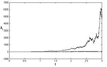
The numerical solution is presented in the graphic for three different trajectories.

Computer implementation
The following Python code implements the Milstein method and uses it to solve the SDE describing geometric Brownian motion defined by
# -*- coding: utf-8 -*-
# Milstein Method
import numpy as np
import matplotlib.pyplot as plt
class Model:
    """Stochastic model constants."""
    mu = 3
    sigma = 1
def dW(dt):
    """Random sample normal distribution."""
    return np.random.normal(loc=0.0, scale=np.sqrt(dt))
def run_simulation():
    """ Return the result of one full simulation."""
    # One second and thousand grid points
    T_INIT = 0
    T_END = 1
    N = 1000 # Compute 1000 grid points
    DT = float(T_END - T_INIT) / N
    TS = np.arange(T_INIT, T_END + DT, DT)
    Y_INIT = 1
    # Vectors to fill
    ys = np.zeros(N + 1)
    ys = Y_INIT
    for i in range(1, TS.size):
        t = (i - 1) * DT
        y = ys
        dw = dW(DT)
        # Sum up terms as in the Milstein method
        ys = y + \
            Model.mu * y * DT + \
            Model.sigma * y * dw + \
            (Model.sigma**2 / 2) * y * (dw**2 - DT)
    return TS, ys
def plot_simulations(num_sims: int):
    """Plot several simulations in one image."""
    for _ in range(num_sims):
        plt.plot(*run_simulation())
    plt.xlabel("time (s)")
    plt.ylabel("y")
    plt.grid()
    plt.show()
if __name__ == "__main__":
    NUM_SIMS = 2
    plot_simulations(NUM_SIMS)
See also
References
- Mil'shtein, G. N. (1974). "Approximate integration of stochastic differential equations". Teoriya Veroyatnostei i ee Primeneniya (in Russian). 19 (3): 583–588.
- Mil’shtein, G. N. (1975). "Approximate Integration of Stochastic Differential Equations". Theory of Probability & Its Applications. 19 (3): 557–000. doi:10.1137/1119062.
- V. Mackevičius, Introduction to Stochastic Analysis, Wiley 2011
- Umberto Picchini, SDE Toolbox: simulation and estimation of stochastic differential equations with Matlab. http://sdetoolbox.sourceforge.net/
Further reading
- Kloeden, P.E., & Platen, E. (1999). Numerical Solution of Stochastic Differential Equations. Springer, Berlin. ISBN 3-540-54062-8.
{{cite book}}: CS1 maint: multiple names: authors list (link)
 with
with  , where
  denotes the
  . Then the Milstein approximation to the true solution
  is the
  defined as follows:
 equal subintervals of width
  :
: 

 for
for  by:
by:  where
where  denotes the
  with respect to
  and:
and:  are
are  . Then
  for
for  , and increasing
  (i.e. the diffusion term does not depend on
  ) this method is equivalent to the
  .
.
 with real constants
  and
and  . Using
 where
where

