Misplaced Pages

In mathematics, a multiplicative cascade is a fractal/multifractal distribution of points produced via an iterative and multiplicative random process.

Definition

The plots above are examples of multiplicative cascade multifractals.

To create these distributions there are a few steps to take. Firstly, we must create a lattice of cells which will be our underlying probability density field.

Secondly, an iterative process is followed to create multiple levels of the lattice: at each iteration the cells are split into four equal parts (cells). Each new cell is then assigned a probability randomly from the set ${\displaystyle \lbrace p_{1},p_{2},p_{3},p_{4}\rbrace }$ without replacement, where ${\displaystyle p_{i}\in }$. This process is continued to the Nth level. For example, in constructing such a model down to level 8 we produce a 4 array of cells.

Thirdly, the cells are filled as follows: We take the probability of a cell being occupied as the product of the cell's own p_i and those of all its parents (up to level 1). A Monte Carlo rejection scheme is used repeatedly until the desired cell population is obtained, as follows: x and y cell coordinates are chosen randomly, and a random number between 0 and 1 is assigned; the (x, y) cell is then populated depending on whether the assigned number is lesser than (outcome: not populated) or greater or equal to (outcome: populated) the cell's occupation probability.

Examples

To produce the plots above we filled the probability density field with 5,000 points in a space of 256 × 256.

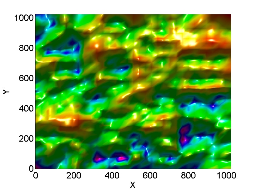
An example of the probability density field:

The fractals are generally not scale-invariant and therefore cannot be considered standard fractals. They can however be considered multifractals. The Rényi (generalized) dimensions can be theoretically predicted. It can be shown that as ${\displaystyle N\rightarrow \infty }$,

${\displaystyle D_{q}={\frac {\log _{2}\left(f_{1}^{q}+f_{2}^{q}+f_{3}^{q}+f_{4}^{q}\right)}{1-q}},}$

where N is the level of the grid refinement and,

${\displaystyle f_{i}={\frac {p_{i}}{\sum _{i}p_{i}}}.}$

See also

• Fractal dimension
• Hausdorff dimension
• Scale invariance

References

1. Meakin, Paul (September 1987). "Diffusion-limited aggregation on multifractal lattices: A model for fluid-fluid displacement in porous media". Physical Review A. 36 (6): 2833–2837. doi:10.1103/PhysRevA.36.2833. PMID 9899187.
2. Cristano G. Sabiu, Luis Teodoro, Martin Hendry, arXiv:0803.3212v1 Resolving the universe with multifractals
3. Martinez et al. ApJ 357 50M "Clustering Paradigms and Multifractal Measures"

• Fractals