| Part of a series on |
| Evolutionary biology |
|---|
 Darwin's finches by John Gould Darwin's finches by John Gould |
| Processes and outcomes |
| Natural history |
| History of evolutionary theory |
Fields and applications
|
| Social implications |
Wagner's gene network model is a computational model of artificial gene networks, which explicitly modeled the developmental and evolutionary process of genetic regulatory networks. A population with multiple organisms can be created and evolved from generation to generation. It was first developed by Andreas Wagner in 1996 and has been investigated by other groups to study the evolution of gene networks, gene expression, robustness, plasticity and epistasis.
Assumptions
The model and its variants have a number of simplifying assumptions. Three of them are listing below.
- The organisms are modeled as gene regulatory networks. The models assume that gene expression is regulated exclusively at the transcriptional level;
- The product of a gene can regulate the expression of (be a regulator of) that source gene or other genes. The models assume that a gene can only produce one active transcriptional regulator;
- The effects of one regulator are independent of effects of other regulators on the same target gene.
Genotype

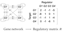
The model represents individuals as networks of interacting transcriptional regulators. Each individual expresses genes encoding transcription factors. The product of each gene can regulate the expression level of itself and/or the other genes through cis-regulatory elements. The interactions among genes constitute a gene network that is represented by a × regulatory matrix in the model. The elements in matrix R represent the interaction strength. Positive values within the matrix represent the activation of the target gene, while negative ones represent repression. Matrix elements with value 0 indicate the absence of interactions between two genes.
Phenotype

The phenotype of each individual is modeled as the gene expression pattern at time . It is represented by a state vector in this model.
whose element denotes the expression state of gene i at time t. In the original Wagner model,
∈
where 1 represents the gene is expressed while -1 implies the gene is not expressed. The expression pattern can only be ON or OFF. The continuous expression pattern between -1 (or 0) and 1 is also implemented in some other variants.
Development
The development process is modeled as the development of gene expression states. The gene expression pattern at time is defined as the initial expression state. The interactions among genes change the expression states during the development process. This process is modeled by the following differential equations
where τ) represents the expression state of at time . It is determined by a filter function σ. represents the weighted sum of regulatory effects () of all genes on gene at time . In the original Wagner model, the filter function is a step function
In other variants, the filter function is implemented as a sigmoidal function
In this way, the expression states will acquire a continuous distribution. The gene expression will reach the final state if it reaches a stable pattern.
Evolution
Evolutionary simulations are performed by reproduction-mutation-selection life cycle. Populations are fixed at size and they will not go extinct. Non-overlapping generations are employed. In a typical evolutionary simulation, a single random viable individual that can produce a stable gene expression pattern is chosen as the founder. Cloned individuals are generated to create a population of identical individuals. According to the asexual or sexual reproductive mode, offspring are produced by randomly choosing (with replacement) parent individual(s) from current generation. Mutations can be acquired with probability μ and survive with probability equal to their fitness. This process is repeated until N individuals are produced that go on to found the following generation.
Fitness
Fitness in this model is the probability that an individual survives to reproduce. In the simplest implementation of the model, developmentally stable genotypes survive (i.e. their fitness is ) and developmentally unstable ones do not (i.e. their fitness is ).
Mutation
Mutations are modeled as the changes in gene regulation, i.e., the changes of the elements in the regulatory matrix .
Reproduction
Both sexual and asexual reproductions are implemented. Asexual reproduction is implemented as producing the offspring's genome (the gene network) by directly copying the parent's genome. Sexual reproduction is implemented as the recombination of the two parents' genomes.
Selection
An organism is considered viable if it reaches a stable gene expression pattern. An organism with oscillated expression pattern is discarded and cannot enter the next generation.
References
- Wagner A (1996). "Does Evolutionary Plasticity Evolve?", Evolution, 50(3):1008-1023.
- ^ Bergman A and Siegal ML (2003). "Evolutionary capacitance as a general feature of complex gene networks", Nature, 424(6948):549-552.
- ^ Azevedo RBR, Lohaus R and Srinivasan S and Dang KK and Burch CL (2006). "Sexual reproduction selects for robustness and negative epistasis in artificial gene networks", Nature, 440(7080):87-90.
- ^ Huerta-Sanchez E, Durrett R (2007). "Wagner's canalization model", Theoretical Population Biology, 71(2):121-130.
 on the right representing the network on the left.
 genes encoding transcription factors. The product of each gene can regulate the expression level of itself and/or the other genes through
  ×
×  in the model. The elements in matrix R represent the interaction strength. Positive values within the matrix represent the activation of the target gene, while negative ones represent repression. Matrix elements with value 0 indicate the absence of interactions between two genes.
 whose elements
  describe the expression states of gene
  .
. . It is represented by a state vector
  in this model.


 at time
  is defined as the initial expression state. The interactions among genes change the expression states during the development process. This process is modeled by the following differential equations

 τ) represents the expression state of
  at time
  . It is determined by a filter function σ
 .
.  represents the weighted sum of regulatory effects (
 ) of all genes on gene
  at time

 ) and developmentally unstable ones do not (i.e. their fitness is
  ).
).