Misplaced Pages

Revision as of 00:53, 24 April 2006

Fisher-Tippett

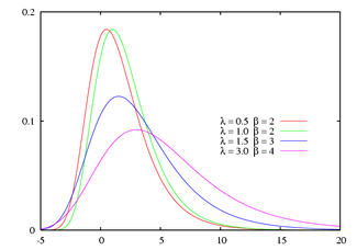
Probability density function
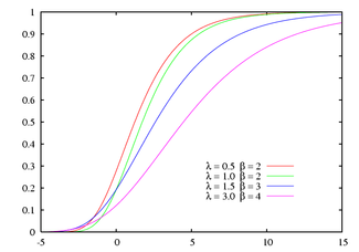
Cumulative distribution function
Parameters	${\displaystyle \mu \!}$ location (real) ${\displaystyle \beta >0\!}$ scale (real)
Support	${\displaystyle x\in (-\infty ;+\infty )\!}$
PDF	${\displaystyle {\frac {\exp(-z)\,z}{\beta }}\!}$ where ${\displaystyle z=\exp \left\!}$
CDF	${\displaystyle \exp(-\exp)\!}$
Mean	${\displaystyle \mu +\beta \,\gamma \!}$
Median	${\displaystyle \mu -\beta \,\ln(\ln(2))\!}$
Mode	${\displaystyle \mu \!}$
Variance	${\displaystyle {\frac {\pi ^{2}}{6}}\,\beta ^{2}\!}$
Skewness	${\displaystyle {\frac {12{\sqrt {6}}\,\zeta (3)}{\pi ^{3}}}\approx 1.14\!}$
Excess kurtosis	${\displaystyle {\frac {12}{5}}}$
Entropy	${\displaystyle \ln(\beta )+\gamma +1\!}$ for ${\displaystyle \beta >\exp(-(\gamma +1))\!}$
MGF	${\displaystyle \Gamma (1-\beta \,t)\,\exp(\mu \,t)\!}$
CF	${\displaystyle \Gamma (1-i\,\beta \,t)\,\exp(i\,\mu \,t)\!}$

In probability theory and statistics the Gumbel distribution (named after Emil Julius Gumbel (1891–1966)) is used to find the minimum (or the maximum) of a number of samples of various distributions. For example we would use it to find the maximum level of a river in a particular year if we had the list of maximum values for the past ten years. It is therefore useful in predicting the chance that an extreme earthquake, flood or other natural disaster will occur.

The distribution of the samples could be of the normal or exponential type. The Gumbel distribution, and similar distributions, are used in extreme value theory.

In particular, the Gumbel distribution is a special case of the Fisher-Tippett distribution (named after Sir Ronald Aylmer Fisher (1890–1962) and Leonard Henry Caleb Tippett (1902–1985)), also known as the log-Weibull distribution.

Properties

The cumulative distribution function is

${\displaystyle F(x;\mu ,\beta )=e^{-e^{(\mu -x)/\beta }}.\,}$

The Gumbel distribution is the case where μ = 0 and β = 1.

The median is ${\displaystyle \mu -\beta \ln(-\ln(0.5))}$

The mean is ${\displaystyle \mu +\gamma \beta }$ where ${\displaystyle \gamma }$ = Euler-Mascheroni constant = 0.57721...

The standard deviation is

${\displaystyle \beta \pi /{\sqrt {6}}.\,}$

The mode is μ.

Parameter estimation

A more practical way of using the distribution could be

${\displaystyle F(x;\mu ,\beta )=e^{-e^{\epsilon (\mu -x)/(\mu -M)}};}$

${\displaystyle \epsilon =\ln(-\ln(0.5))=-0.367...\,}$

where M is the median. To fit values one could get the median straight away and then vary μ until it fits the list of values.

Generating Fisher-Tippett variates

Given a random variate U drawn from the uniform distribution in the interval (0, 1], the variate

${\displaystyle X=\mu -\beta \ln(-\ln(U))\,}$

has a Fisher-Tippett distribution with parameters μ and β. This follows from the form of the cumulative distribution function given above.

See also

• order statistic

• Continuous distributions