Misplaced Pages

Revision as of 14:28, 27 November 2011

Shifted Gompertz

Probability density function
Cumulative distribution function
Parameters	${\displaystyle b>0}$ scale (real) ${\displaystyle \eta >0}$ shape (real)
Support	${\displaystyle x\in \mathbb {R} ^{+}}$
PDF	${\displaystyle be^{-bx}e^{-\eta e^{-bx}}\left}$
CDF	${\displaystyle \left(1-e^{-bx}\right)e^{-\eta e^{-bx}}}$
Mean	${\displaystyle (-1/b)\{\mathrm {E} -\ln(\eta )\}\,}$ where ${\displaystyle X=\eta e^{-bx}\,}$ and ${\displaystyle {\begin{aligned}\mathrm {E} =&\!\!\int _{0}^{\eta }\!\!\!\!e^{-X}dX\\&-1/\eta \!\!\int _{0}^{\eta }\!\!\!\!Xe^{-X}dX\end{aligned}}}$
Mode	${\displaystyle 0\,}$ for ${\displaystyle \eta \leq 0.5\,}$, ${\displaystyle (-1/b)\ln(z^{\star })\,}$ for ${\displaystyle \eta >0.5\,}$where${\displaystyle z^{\star }=/(2\eta )}$
Variance	${\displaystyle (1/b^{2})(\mathrm {E} \{^{2}\}-(\mathrm {E} )^{2})\,}$ where ${\displaystyle X=\eta e^{-bx}\,}$ and ${\displaystyle {\begin{aligned}\mathrm {E} \{^{2}\}=&\!\!\int _{0}^{\eta }\!\!\!\!e^{-X}^{2}\,dX\\&{}-1/\eta \!\!\int _{0}^{\eta }\!\!\!\!Xe^{-X}^{2}\,dX\end{aligned}}}$

The Gompertz distribution is an extreme value (reverted Gumbel distribution) distribution which is truncated at zero. It has been used as a model of customer lifetime.

Specification

Probability density function

The probability density function of the Gompertz distribution is:

${\displaystyle f(x;b,\eta )=be^{-bx}e^{-\eta e^{-bx}}\left\mathrm {for} \ x>0\,\!}$

where ${\displaystyle b>0}$ is the scale parameter and ${\displaystyle \eta >0}$ is the shape parameter of the Gompertz distribution.

Cumulative distribution function

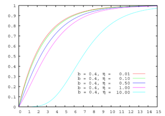
The cumulative distribution function of the Gompertz distribution is:

${\displaystyle F(x;b,\eta )=\left(1-e^{-bx}\right)e^{-\eta e^{-bx}}\mathrm {for} \ x>0.\,\!}$

Properties

The Gompertz distribution is right-skewed for all values of ${\displaystyle \eta }$.

Shapes

The Gompertz density function can take on different shapes depending on the values of the shape parameter ${\displaystyle \eta }$:

• ${\displaystyle \eta \geq 1\,}$ the probability density function has its mode at 0.
• ${\displaystyle \eta <1\,}$ the probability density function has its mode at

Failed to parse (unknown function "\x"): {\displaystyle \x*}=-\frac{\ln(z^\star)}{b}\, \qquad 0 < z^\star < 1}

where ${\displaystyle z^{\star }\,}$ is the smallest root of

${\displaystyle \eta ^{2}z^{2}-\eta (3+\eta )z+\eta +1=0\,,}$

which is

${\displaystyle z^{\star }=/(2\eta ).}$

Related distributions

The Gompertz distribution is a natural conjugate to a gamma distribution. If ${\displaystyle \eta }$ varies according to a gamma distribution with shape parameter ${\displaystyle \alpha }$ and scale parameter ${\displaystyle \beta }$ (mean = ${\displaystyle \alpha \beta }$), the cumulative distribution function is Gamma/Gompertz (G/G).

See also

• Gompertz function
• Gompertz–Makeham law of mortality

• Continuous distributions