Misplaced Pages

This is an old revision of this page, as edited by 141.228.106.149 (talk) at 11:06, 8 November 2011 (→Parameter estimation). The present address (URL) is a permanent link to this revision, which may differ significantly from the current revision.

Gumbel

Probability density function
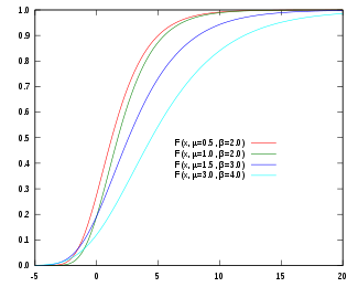
Cumulative distribution function
Parameters	${\displaystyle \mu \!}$ location (real) ${\displaystyle \beta >0\!}$ scale (real)
Support	${\displaystyle x\in (-\infty ;+\infty )\!}$
PDF	${\displaystyle {\frac {1}{\beta }}e^{-z-e^{-z}}\!}$ where ${\displaystyle z={\frac {x-\mu }{\beta }}\!}$
CDF	${\displaystyle \exp(-e^{-(x-\mu )/\beta })\!}$
Mean	${\displaystyle \mu +\beta \,\gamma \!}$
Median	${\displaystyle \mu -\beta \,\ln(\ln(2))\!}$
Mode	${\displaystyle \mu \!}$
Variance	${\displaystyle {\frac {\pi ^{2}}{6}}\,\beta ^{2}\!}$
Skewness	${\displaystyle {\frac {12{\sqrt {6}}\,\zeta (3)}{\pi ^{3}}}\approx 1.14\!}$
Excess kurtosis	${\displaystyle {\frac {12}{5}}}$
Entropy	${\displaystyle \ln(\beta )+\gamma +1\!}$
MGF	${\displaystyle \Gamma (1-\beta \,t)\,e^{\mu \,t}\!}$
CF	${\displaystyle \Gamma (1-i\,\beta \,t)\,e^{i\,\mu \,t}\!}$

In probability theory and statistics, the Gumbel distribution (named after Emil Julius Gumbel (1891–1966)) is used to model the distribution of the maximum (or the minimum) of a number of samples of various distributions. For example we would use it to represent the distribution of the maximum level of a river in a particular year if we had the list of maximum values for the past ten years. It is useful in predicting the chance that an extreme earthquake, flood or other natural disaster will occur.

The potential applicability of the Gumbel distribution to represent the distribution of maxima relates to extreme value theory which indicates that it is likely to be useful if the distribution of the underlying sample data is of the normal or exponential type.

The Gumbel distribution is a particular case of generalized extreme value distribution (also known as the Fisher-Tippett distribution) and the distribution is also known as the log-Weibull distribution and the double exponential distribution (which is sometimes used to refer to the Laplace distribution).

Properties

The cumulative distribution function of the Gumbel distribution is

${\displaystyle F(x;\mu ,\beta )=e^{-e^{-(x-\mu )/\beta }}.\,}$

The median is ${\displaystyle \mu -\beta \ln \left(\ln 2\right)}$

The mean is ${\displaystyle \mu +\gamma \beta }$ where ${\displaystyle \gamma }$ = Euler–Mascheroni constant ${\displaystyle \approx }$ 0.5772156649015328606.

The standard deviation is

${\displaystyle \beta \pi /{\sqrt {6}}.\,}$

The mode is μ.

Standard Gumbel distribution

The standard Gumbel distribution is the case where μ = 0 and β = 1 with cumulative distribution function

${\displaystyle F(x)=e^{-e^{(-x)}}\,}$

and probability density function

${\displaystyle f(x)=e^{-x}e^{-e^{-x}}.}$

The median is ${\displaystyle -\ln(\ln(2))\approx }$ 0.36651292058166432701.

The mean is ${\displaystyle \gamma }$, the Euler–Mascheroni constant ${\displaystyle \approx }$ 0.5772156649015328606.

The standard deviation is

${\displaystyle \pi /{\sqrt {6}}\approx }$ 1.28254983016186409554.

The mode is 0.

Parameter estimation

A more practical way of using the distribution could be

${\displaystyle F(x;\mu ,\beta )=e^{-e^{\varepsilon (\mu -x)/(\mu -M)}};}$

${\displaystyle \varepsilon =\ln(\ln(2))=-0.367\dots \,}$

where M is the median. To fit values one could get the median straight away and then vary μ until it fits the list of values.

Generating Gumbel variates

Given a random variate U drawn from the uniform distribution in the interval , the variate

${\displaystyle X=\mu -\beta \ln(-\ln(U))\,}$

has a Gumbel distribution with parameters μ and β. This follows from the form of the cumulative distribution function given above.

Related distributions

When the cdf of Y is the converse of the Gumbel standard cumulative distribution, ${\displaystyle P(Y\leq y)=1-F(y)}$, then Y has a Gompertz distribution.

Application

Gumbel has shown that the maximum value (or first order statistic) in a sample of a random variable following an exponential distribution approaches the Gumbel distribution closer with increasing sample size.

In hydrology, therefore, the Gumbel distribution is used to analyze such variables as monthly and annual maximum values of daily rainfall and river discharge volumes.

Gumbel has also shown that the estimator r / (n+1) for the probability of an event - where r is the rank number of the observed value in the data series and n is the total number of observations - is an unbiased estimator of the cumulative probability around the mode of the distribution. Therefore, this estimator is often used as a plotting position.

The blue picture illustrates an example of fitting the Gumbel distribution to ranked maximum one-day October rainfalls showing also the 90% confidence belt based on the binomial distribution. The rainfall data are represented by the plotting position r / (n+1) as part of the cumulative frequency analysis.

See also

• Type-1 Gumbel distribution
• Type-2 Gumbel distribution
• Extreme value theory
• Generalized extreme value distribution
• Fisher–Tippett–Gnedenko theorem
• CumFreq (application software for probability distributions including Gumbel)

References

1. Willemse, W. J. and Kaas, R., "Rational reconstruction of frailty-based mortality models by a generalisation of Gompertz’ law of mortality", Insurance: Mathematics and Economics, 40 (3) (2007), 468–484.
2. Gumbel, E.J. 1954. Statistical theory of extreme values and some practical applications. Applied mathematics series 33. U.S. Department of Commerce, National Bureau of Standards.
3. Ritzema (ed.), H.P. (1994). Frequency and Regression Analysis (PDF). Chapter 6 in: Drainage Principles and Applications, Publication 16, International Institute for Land Reclamation and Improvement (ILRI), Wageningen, The Netherlands. pp. 175–224. ISBN 90 70754 3 39. {{cite book}}: |last= has generic name (help)

• Continuous distributions
• Extreme value data