| Part of a series on statistics |
| Probability theory |
|---|
 |

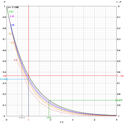
Blue curve: Throwing a 6-sided die 6 times gives a 33.5% chance that 6 (or any other given number) never turns up; it can be observed that as n increases, the probability of a 1/n-chance event never appearing after n tries rapidly converges to 0.
Grey curve: To get 50-50 chance of throwing a Yahtzee (5 cubic dice all showing the same number) requires 0.69 × 1296 ~ 898 throws.
Green curve: Drawing a card from a deck of playing cards without jokers 100 (1.92 × 52) times with replacement gives 85.7% chance of drawing the ace of spades at least once.
In the theory of probability and statistics, a Bernoulli trial (or binomial trial) is a random experiment with exactly two possible outcomes, "success" and "failure", in which the probability of success is the same every time the experiment is conducted. It is named after Jacob Bernoulli, a 17th-century Swiss mathematician, who analyzed them in his Ars Conjectandi (1713).
The mathematical formalization and advanced formulation of the Bernoulli trial is known as the Bernoulli process.
Since a Bernoulli trial has only two possible outcomes, it can be framed as a "yes or no" question. For example:
- Is the top card of a shuffled deck an ace?
- Was the newborn child a girl? (See human sex ratio.)
Success and failure are in this context labels for the two outcomes, and should not be construed literally or as value judgments. More generally, given any probability space, for any event (set of outcomes), one can define a Bernoulli trial according to whether the event occurred or not (event or complementary event). Examples of Bernoulli trials include:
- Flipping a coin. In this context, obverse ("heads") conventionally denotes success and reverse ("tails") denotes failure. A fair coin has the probability of success 0.5 by definition. In this case, there are exactly two possible outcomes.
- Rolling a ‹See Tfd›die, where a six is "success" and everything else a "failure". In this case, there are six possible outcomes, and the event is a six; the complementary event "not a six" corresponds to the other five possible outcomes.
- In conducting a political opinion poll, choosing a voter at random to ascertain whether that voter will vote "yes" in an upcoming referendum.
Definition
Independent repeated trials of an experiment with exactly two possible outcomes are called Bernoulli trials. Call one of the outcomes "success" and the other outcome "failure". Let be the probability of success in a Bernoulli trial, and be the probability of failure. Then the probability of success and the probability of failure sum to one, since these are complementary events: "success" and "failure" are mutually exclusive and exhaustive. Thus, one has the following relations:
Alternatively, these can be stated in terms of odds: given probability of success and of failure, the odds for are and the odds against are These can also be expressed as numbers, by dividing, yielding the odds for, , and the odds against, :
These are multiplicative inverses, so they multiply to 1, with the following relations:
In the case that a Bernoulli trial is representing an event from finitely many equally likely outcomes, where of the outcomes are success and of the outcomes are failure, the odds for are and the odds against are This yields the following formulas for probability and odds:
Here the odds are computed by dividing the number of outcomes, not the probabilities, but the proportion is the same, since these ratios only differ by multiplying both terms by the same constant factor.
Random variables describing Bernoulli trials are often encoded using the convention that 1 = "success", 0 = "failure".
Closely related to a Bernoulli trial is a binomial experiment, which consists of a fixed number of statistically independent Bernoulli trials, each with a probability of success , and counts the number of successes. A random variable corresponding to a binomial experiment is denoted by , and is said to have a binomial distribution. The probability of exactly successes in the experiment is given by:
where is a binomial coefficient.
Bernoulli trials may also lead to negative binomial distributions (which count the number of successes in a series of repeated Bernoulli trials until a specified number of failures are seen), as well as various other distributions.
When multiple Bernoulli trials are performed, each with its own probability of success, these are sometimes referred to as Poisson trials.
Examples
Tossing coins
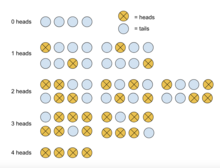
Consider the simple experiment where a fair coin is tossed four times. Find the probability that exactly two of the tosses result in heads.
Solution

For this experiment, let a heads be defined as a success and a tails as a failure. Because the coin is assumed to be fair, the probability of success is . Thus, the probability of failure, , is given by
- .
Using the equation above, the probability of exactly two tosses out of four total tosses resulting in a heads is given by:
Rolling dice
What is probability that when three independent fair six-sided dice are rolled, exactly two yield sixes?
Solution

On one die, the probability of rolling a six, . Thus, the probability of not rolling a six, .
As above, the probability of exactly two sixes out of three,
See also
- Bernoulli scheme
- Bernoulli sampling
- Bernoulli distribution
- Binomial distribution
- Binomial coefficient
- Binomial proportion confidence interval
- Poisson sampling
- Sampling design
- Coin flipping
- Jacob Bernoulli
- Fisher's exact test
- Boschloo's test
References
- Papoulis, A. (1984). "Bernoulli Trials". Probability, Random Variables, and Stochastic Processes (2nd ed.). New York: McGraw-Hill. pp. 57–63.
- James Victor Uspensky: Introduction to Mathematical Probability, McGraw-Hill, New York 1937, page 45
- Rajeev Motwani and P. Raghavan. Randomized Algorithms. Cambridge University Press, New York (NY), 1995, p.67-68
External links
- "Bernoulli trials", Encyclopedia of Mathematics, EMS Press, 2001
- "Simulation of n Bernoulli trials". math.uah.edu. Retrieved 2014-01-21.
 be the probability of success in a Bernoulli trial, and
  be the probability of failure. Then the probability of success and the probability of failure sum to one, since these are complementary events: "success" and "failure" are
 and the odds against are
  These can also be expressed as numbers, by dividing, yielding the odds for,
  , and the odds against,
  :
:


 of the outcomes are success and
  of the outcomes are failure, the odds for are
  and the odds against are
  This yields the following formulas for probability and odds:

 of
of  , and is said to have a
  successes in the experiment
 is a
is a  . Thus, the probability of failure,
  .
.
 . Thus, the probability of not rolling a six,
  .
.
