Misplaced Pages

Beta prime

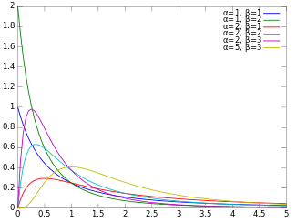
Probability density function
Cumulative distribution function
Parameters	${\displaystyle \alpha >0}$ shape (real) ${\displaystyle \beta >0}$ shape (real)
Support	${\displaystyle x\in [0,\infty )\!}$
PDF	${\displaystyle f(x)={\frac {x^{\alpha -1}(1+x)^{-\alpha -\beta }}{\mathrm {B} (\alpha ,\beta )}}\!}$
CDF	${\displaystyle I_{{\frac {x}{1+x}}(\alpha ,\beta )}}$ where ${\displaystyle I_{x}(\alpha ,\beta )}$ is the incomplete beta function
Mean	${\displaystyle {\frac {\alpha }{\beta -1}}}$ if ${\displaystyle \beta >1}$
Mode	${\displaystyle {\frac {\alpha -1}{\beta +1}}{\text{ if }}\alpha \geq 1{\text{, 0 otherwise}}\!}$
Variance	${\displaystyle {\frac {\alpha (\alpha +\beta -1)}{(\beta -2)(\beta -1)^{2}}}}$ if ${\displaystyle \beta >2}$
Skewness	${\displaystyle {\frac {2(2\alpha +\beta -1)}{\beta -3}}{\sqrt {\frac {\beta -2}{\alpha (\alpha +\beta -1)}}}}$ if ${\displaystyle \beta >3}$
Excess kurtosis	${\displaystyle 6{\frac {\alpha (\alpha +\beta -1)(5\beta -11)+(\beta -1)^{2}(\beta -2)}{\alpha (\alpha +\beta -1)(\beta -3)(\beta -4)}}}$ if ${\displaystyle \beta >4}$
Entropy	${\displaystyle {\begin{aligned}&\log \left(\mathrm {B} (\alpha ,\beta )\right)+(\alpha -1)(\psi (\beta )-\psi (\alpha ))\\+&(\alpha +\beta )\left(\psi (1-\alpha -\beta )-\psi (1-\beta )+{\frac {\pi \sin(\alpha \pi )}{\sin(\beta \pi )\sin((\alpha +\beta )\pi ))}}\right)\end{aligned}}}$ where ${\displaystyle \psi }$ is the digamma function.
MGF	Does not exist
CF	${\displaystyle {\frac {e^{-it}\Gamma (\alpha +\beta )}{\Gamma (\beta )}}G_{1,2}^{\,2,0}\!\left(\left.{\begin{matrix}\alpha +\beta \\\beta ,0\end{matrix}}\;\right|\,-it\right)}$

In probability theory and statistics, the beta prime distribution (also known as inverted beta distribution or beta distribution of the second kind) is an absolutely continuous probability distribution. If ${\displaystyle p\in }$ has a beta distribution, then the odds ${\displaystyle {\frac {p}{1-p}}}$ has a beta prime distribution.

Definitions

Beta prime distribution is defined for ${\displaystyle x>0}$ with two parameters α and β, having the probability density function:

${\displaystyle f(x)={\frac {x^{\alpha -1}(1+x)^{-\alpha -\beta }}{\mathrm {B} (\alpha ,\beta )}}}$

where B is the Beta function.

The cumulative distribution function is

${\displaystyle F(x;\alpha ,\beta )=I_{\frac {x}{1+x}}\left(\alpha ,\beta \right),}$

where I is the regularized incomplete beta function.

While the related beta distribution is the conjugate prior distribution of the parameter of a Bernoulli distribution expressed as a probability, the beta prime distribution is the conjugate prior distribution of the parameter of a Bernoulli distribution expressed in odds. The distribution is a Pearson type VI distribution.

The mode of a variate X distributed as ${\displaystyle \beta '(\alpha ,\beta )}$ is ${\displaystyle {\hat {X}}={\frac {\alpha -1}{\beta +1}}}$. Its mean is ${\displaystyle {\frac {\alpha }{\beta -1}}}$ if ${\displaystyle \beta >1}$ (if ${\displaystyle \beta \leq 1}$ the mean is infinite, in other words it has no well defined mean) and its variance is ${\displaystyle {\frac {\alpha (\alpha +\beta -1)}{(\beta -2)(\beta -1)^{2}}}}$ if ${\displaystyle \beta >2}$.

For ${\displaystyle -\alpha <k<\beta }$, the k-th moment ${\displaystyle E}$ is given by

${\displaystyle E={\frac {\mathrm {B} (\alpha +k,\beta -k)}{\mathrm {B} (\alpha ,\beta )}}.}$

For ${\displaystyle k\in \mathbb {N} }$ with ${\displaystyle k<\beta ,}$ this simplifies to

${\displaystyle E=\prod _{i=1}^{k}{\frac {\alpha +i-1}{\beta -i}}.}$

The cdf can also be written as

${\displaystyle {\frac {x^{\alpha }\cdot {}_{2}F_{1}(\alpha ,\alpha +\beta ,\alpha +1,-x)}{\alpha \cdot \mathrm {B} (\alpha ,\beta )}}}$

where ${\displaystyle {}_{2}F_{1}}$ is the Gauss's hypergeometric function ₂F₁ .

Alternative parameterization

The beta prime distribution may also be reparameterized in terms of its mean μ > 0 and precision ν > 0 parameters ( p. 36).

Consider the parameterization μ = α/(β − 1) and ν = β − 2, i.e., α = μ(1 + ν) and β = 2 + ν. Under this parameterization E = μ and Var = μ(1 + μ)/ν.

Generalization

Two more parameters can be added to form the generalized beta prime distribution ${\displaystyle \beta '(\alpha ,\beta ,p,q)}$:

• ${\displaystyle p>0}$ shape (real)
• ${\displaystyle q>0}$ scale (real)

having the probability density function:

${\displaystyle f(x;\alpha ,\beta ,p,q)={\frac {p\left({\frac {x}{q}}\right)^{\alpha p-1}\left(1+\left({\frac {x}{q}}\right)^{p}\right)^{-\alpha -\beta }}{q\mathrm {B} (\alpha ,\beta )}}}$

with mean

${\displaystyle {\frac {q\Gamma \left(\alpha +{\tfrac {1}{p}}\right)\Gamma (\beta -{\tfrac {1}{p}})}{\Gamma (\alpha )\Gamma (\beta )}}\quad {\text{if }}\beta p>1}$

and mode

${\displaystyle q\left({\frac {\alpha p-1}{\beta p+1}}\right)^{\tfrac {1}{p}}\quad {\text{if }}\alpha p\geq 1}$

Note that if p = q = 1 then the generalized beta prime distribution reduces to the standard beta prime distribution.

This generalization can be obtained via the following invertible transformation. If ${\displaystyle y\sim \beta '(\alpha ,\beta )}$ and ${\displaystyle x=qy^{1/p}}$ for ${\displaystyle q,p>0}$, then ${\displaystyle x\sim \beta '(\alpha ,\beta ,p,q)}$.

Compound gamma distribution

The compound gamma distribution is the generalization of the beta prime when the scale parameter, q is added, but where p = 1. It is so named because it is formed by compounding two gamma distributions:

${\displaystyle \beta '(x;\alpha ,\beta ,1,q)=\int _{0}^{\infty }G(x;\alpha ,r)G(r;\beta ,q)\;dr}$

where ${\displaystyle G(x;a,b)}$ is the gamma pdf with shape ${\displaystyle a}$ and inverse scale ${\displaystyle b}$.

The mode, mean and variance of the compound gamma can be obtained by multiplying the mode and mean in the above infobox by q and the variance by q.

Another way to express the compounding is if ${\displaystyle r\sim G(\beta ,q)}$ and ${\displaystyle x\mid r\sim G(\alpha ,r)}$, then ${\displaystyle x\sim \beta '(\alpha ,\beta ,1,q)}$. This gives one way to generate random variates with compound gamma, or beta prime distributions. Another is via the ratio of independent gamma variates, as shown below.

Properties

• If ${\displaystyle X\sim \beta '(\alpha ,\beta )}$ then ${\displaystyle {\tfrac {1}{X}}\sim \beta '(\beta ,\alpha )}$.
• If ${\displaystyle Y\sim \beta '(\alpha ,\beta )}$, and ${\displaystyle X=qY^{1/p}}$, then ${\displaystyle X\sim \beta '(\alpha ,\beta ,p,q)}$.
• If ${\displaystyle X\sim \beta '(\alpha ,\beta ,p,q)}$ then ${\displaystyle kX\sim \beta '(\alpha ,\beta ,p,kq)}$.
• ${\displaystyle \beta '(\alpha ,\beta ,1,1)=\beta '(\alpha ,\beta )}$

Related distributions

• If ${\displaystyle X\sim {\textrm {Beta}}(\alpha ,\beta )}$, then ${\displaystyle {\frac {X}{1-X}}\sim \beta '(\alpha ,\beta )}$. This property can be used to generate beta prime distributed variates.
• If ${\displaystyle X\sim \beta '(\alpha ,\beta )}$, then ${\displaystyle {\frac {X}{1+X}}\sim {\textrm {Beta}}(\alpha ,\beta )}$. This is a corollary from the property above.
• If ${\displaystyle X\sim F(2\alpha ,2\beta )}$ has an F-distribution, then ${\displaystyle {\tfrac {\alpha }{\beta }}X\sim \beta '(\alpha ,\beta )}$, or equivalently, ${\displaystyle X\sim \beta '(\alpha ,\beta ,1,{\tfrac {\beta }{\alpha }})}$.
• For gamma distribution parametrization I:
  • If ${\displaystyle X_{k}\sim \Gamma (\alpha _{k},\theta _{k})}$ are independent, then ${\displaystyle {\tfrac {X_{1}}{X_{2}}}\sim \beta '(\alpha _{1},\alpha _{2},1,{\tfrac {\theta _{1}}{\theta _{2}}})}$. Note ${\displaystyle \theta _{1},\theta _{2},{\tfrac {\theta _{1}}{\theta _{2}}}}$ are all scale parameters for their respective distributions.
• For gamma distribution parametrization II:
  • If ${\displaystyle X_{k}\sim \Gamma (\alpha _{k},\beta _{k})}$ are independent, then ${\displaystyle {\tfrac {X_{1}}{X_{2}}}\sim \beta '(\alpha _{1},\alpha _{2},1,{\tfrac {\beta _{2}}{\beta _{1}}})}$. The ${\displaystyle \beta _{k}}$ are rate parameters, while ${\displaystyle {\tfrac {\beta _{2}}{\beta _{1}}}}$ is a scale parameter.
  • If ${\displaystyle \beta _{2}\sim \Gamma (\alpha _{1},\beta _{1})}$ and ${\displaystyle X_{2}\mid \beta _{2}\sim \Gamma (\alpha _{2},\beta _{2})}$, then ${\displaystyle X_{2}\sim \beta '(\alpha _{2},\alpha _{1},1,\beta _{1})}$. The ${\displaystyle \beta _{k}}$ are rate parameters for the gamma distributions, but ${\displaystyle \beta _{1}}$ is the scale parameter for the beta prime.
• ${\displaystyle \beta '(p,1,a,b)={\textrm {Dagum}}(p,a,b)}$ the Dagum distribution
• ${\displaystyle \beta '(1,p,a,b)={\textrm {SinghMaddala}}(p,a,b)}$ the Singh–Maddala distribution.
• ${\displaystyle \beta '(1,1,\gamma ,\sigma )={\textrm {LL}}(\gamma ,\sigma )}$ the log logistic distribution.
• The beta prime distribution is a special case of the type 6 Pearson distribution.
• If X has a Pareto distribution with minimum ${\displaystyle x_{m}}$ and shape parameter ${\displaystyle \alpha }$, then ${\displaystyle {\dfrac {X}{x_{m}}}-1\sim \beta ^{\prime }(1,\alpha )}$.
• If X has a Lomax distribution, also known as a Pareto Type II distribution, with shape parameter ${\displaystyle \alpha }$ and scale parameter ${\displaystyle \lambda }$, then ${\displaystyle {\frac {X}{\lambda }}\sim \beta ^{\prime }(1,\alpha )}$.
• If X has a standard Pareto Type IV distribution with shape parameter ${\displaystyle \alpha }$ and inequality parameter ${\displaystyle \gamma }$, then ${\displaystyle X^{\frac {1}{\gamma }}\sim \beta ^{\prime }(1,\alpha )}$, or equivalently, ${\displaystyle X\sim \beta ^{\prime }(1,\alpha ,{\tfrac {1}{\gamma }},1)}$.
• The inverted Dirichlet distribution is a generalization of the beta prime distribution.
• If ${\displaystyle X\sim \beta '(\alpha ,\beta )}$, then ${\displaystyle \ln X}$ has a generalized logistic distribution. More generally, if ${\displaystyle X\sim \beta '(\alpha ,\beta ,p,q)}$, then ${\displaystyle \ln X}$ has a scaled and shifted generalized logistic distribution.
• If ${\displaystyle X\sim \beta '\left({\frac {1}{2}},{\frac {1}{2}}\right)}$, then ${\displaystyle \pm {\sqrt {X}}}$ follows a Cauchy distribution, which is equivalent to a student-t distribution with the degrees of freedom of 1.

Notes

1. ^ Johnson et al (1995), p 248
2. Bourguignon, M.; Santos-Neto, M.; de Castro, M. (2021). "A new regression model for positive random variables with skewed and long tail". Metron. 79: 33–55. doi:10.1007/s40300-021-00203-y. S2CID 233534544.
3. Dubey, Satya D. (December 1970). "Compound gamma, beta and F distributions". Metrika. 16: 27–31. doi:10.1007/BF02613934. S2CID 123366328.

References

• Johnson, N.L., Kotz, S., Balakrishnan, N. (1995). Continuous Univariate Distributions, Volume 2 (2nd Edition), Wiley. ISBN 0-471-58494-0
• Bourguignon, M.; Santos-Neto, M.; de Castro, M. (2021), "A new regression model for positive random variables with skewed and long tail", Metron, 79: 33–55, doi:10.1007/s40300-021-00203-y, S2CID 233534544

• MathWorld article

• Continuous distributions
• Compound probability distributions