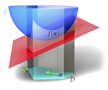
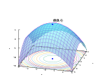
The Frank–Wolfe algorithm is an iterative first-order optimization algorithm for constrained convex optimization. Also known as the conditional gradient method, reduced gradient algorithm and the convex combination algorithm, the method was originally proposed by Marguerite Frank and Philip Wolfe in 1956. In each iteration, the Frank–Wolfe algorithm considers a linear approximation of the objective function, and moves towards a minimizer of this linear function (taken over the same domain).
Problem statement
Suppose is a compact convex set in a vector space and is a convex, differentiable real-valued function. The Frank–Wolfe algorithm solves the optimization problem
- Minimize
- subject to .
Algorithm

- Initialization: Let , and let be any point in .
- Step 1. Direction-finding subproblem: Find solving
- Minimize
- Subject to
- (Interpretation: Minimize the linear approximation of the problem given by the first-order Taylor approximation of around constrained to stay within .)
- Step 2. Step size determination: Set , or alternatively find that minimizes subject to .
- Step 3. Update: Let , let and go to Step 1.
Properties
While competing methods such as gradient descent for constrained optimization require a projection step back to the feasible set in each iteration, the Frank–Wolfe algorithm only needs the solution of a convex problem over the same set in each iteration, and automatically stays in the feasible set.
The convergence of the Frank–Wolfe algorithm is sublinear in general: the error in the objective function to the optimum is after k iterations, so long as the gradient is Lipschitz continuous with respect to some norm. The same convergence rate can also be shown if the sub-problems are only solved approximately.
The iterations of the algorithm can always be represented as a sparse convex combination of the extreme points of the feasible set, which has helped to the popularity of the algorithm for sparse greedy optimization in machine learning and signal processing problems, as well as for example the optimization of minimum–cost flows in transportation networks.
If the feasible set is given by a set of linear constraints, then the subproblem to be solved in each iteration becomes a linear program.
While the worst-case convergence rate with can not be improved in general, faster convergence can be obtained for special problem classes, such as some strongly convex problems.
Lower bounds on the solution value, and primal-dual analysis
Since is convex, for any two points we have:
This also holds for the (unknown) optimal solution . That is, . The best lower bound with respect to a given point is given by
The latter optimization problem is solved in every iteration of the Frank–Wolfe algorithm, therefore the solution of the direction-finding subproblem of the -th iteration can be used to determine increasing lower bounds during each iteration by setting and
Such lower bounds on the unknown optimal value are important in practice because they can be used as a stopping criterion, and give an efficient certificate of the approximation quality in every iteration, since always .
It has been shown that this corresponding duality gap, that is the difference between and the lower bound , decreases with the same convergence rate, i.e.
Notes
- Levitin, E. S.; Polyak, B. T. (1966). "Constrained minimization methods". USSR Computational Mathematics and Mathematical Physics. 6 (5): 1. doi:10.1016/0041-5553(66)90114-5.
- Frank, M.; Wolfe, P. (1956). "An algorithm for quadratic programming". Naval Research Logistics Quarterly. 3 (1–2): 95–110. doi:10.1002/nav.3800030109.
- Dunn, J. C.; Harshbarger, S. (1978). "Conditional gradient algorithms with open loop step size rules". Journal of Mathematical Analysis and Applications. 62 (2): 432. doi:10.1016/0022-247X(78)90137-3.
- Clarkson, K. L. (2010). "Coresets, sparse greedy approximation, and the Frank-Wolfe algorithm". ACM Transactions on Algorithms. 6 (4): 1–30. CiteSeerX 10.1.1.145.9299. doi:10.1145/1824777.1824783.
- Fukushima, M. (1984). "A modified Frank-Wolfe algorithm for solving the traffic assignment problem". Transportation Research Part B: Methodological. 18 (2): 169–177. doi:10.1016/0191-2615(84)90029-8.
- Bertsekas, Dimitri (1999). Nonlinear Programming. Athena Scientific. p. 215. ISBN 978-1-886529-00-7.
Bibliography
- Jaggi, Martin (2013). "Revisiting Frank–Wolfe: Projection-Free Sparse Convex Optimization". Journal of Machine Learning Research: Workshop and Conference Proceedings. 28 (1): 427–435. (Overview paper)
- The Frank–Wolfe algorithm description
- Nocedal, Jorge; Wright, Stephen J. (2006). Numerical Optimization (2nd ed.). Berlin, New York: Springer-Verlag. ISBN 978-0-387-30303-1..
External links
- https://conditional-gradients.org/: a survey of Frank–Wolfe algorithms.
- Marguerite Frank giving a personal account of the history of the algorithm
See also
| Optimization: Algorithms, methods, and heuristics | ||||||||||||||||||
|---|---|---|---|---|---|---|---|---|---|---|---|---|---|---|---|---|---|---|
|  | |||||||||||||||||
|
| ||||||||||||||||||
| ||||||||||||||||||
| ||||||||||||||||||
 is a
is a  is a
is a 
 .
. , and let
  be any point in
  solving


 around
  constrained to stay within
  , or alternatively find
  that minimizes
  subject to
  .
. , let
, let  and go to Step 1.
 after k iterations, so long as the gradient is
  we have:

 . That is,
  . The best lower bound with respect to a given point
  is given by

 -th iteration can be used to determine increasing lower bounds
  during each iteration by setting
  and
and

 .
.
 and the lower bound