In algebraic geometry, a quartic plane curve is a plane algebraic curve of the fourth degree. It can be defined by a bivariate quartic equation:
with at least one of A, B, C, D, E not equal to zero. This equation has 15 constants. However, it can be multiplied by any non-zero constant without changing the curve; thus by the choice of an appropriate constant of multiplication, any one of the coefficients can be set to 1, leaving only 14 constants. Therefore, the space of quartic curves can be identified with the real projective space It also follows, from Cramer's theorem on algebraic curves, that there is exactly one quartic curve that passes through a set of 14 distinct points in general position, since a quartic has 14 degrees of freedom.
A quartic curve can have a maximum of:
- Four connected components
- Twenty-eight bi-tangents
- Three ordinary double points.
One may also consider quartic curves over other fields (or even rings), for instance the complex numbers. In this way, one gets Riemann surfaces, which are one-dimensional objects over but are two-dimensional over An example is the Klein quartic. Additionally, one can look at curves in the projective plane, given by homogeneous polynomials.
Examples
Various combinations of coefficients in the above equation give rise to various important families of curves as listed below.
|
|
-
 Ampersand curve
-
 Bean curve
-
 Bicuspid curve
-
 Bow curve
-
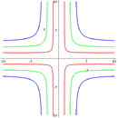
 Cruciform curve with parameters (b,a) being (1,1) in red; (2,2) in green; (3,3) in blue.
-
 Cruciform curve with parameters (b,a) being (1,1) in red; (2,1) in green; (3,1) in blue.
-
 Spiric section
-
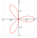
 Three-leaved clover in Cartesian coordinates
-
 Three-leaved clover in polar coordinates
Ampersand curve
The ampersand curve is a quartic plane curve given by the equation:
It has genus zero, with three ordinary double points, all in the real plane.
Bean curve
The bean curve is a quartic plane curve with the equation:
The bean curve has genus zero. It has one singularity at the origin, an ordinary triple point.
Bicuspid curve
The bicuspid is a quartic plane curve with the equation
where a determines the size of the curve. The bicuspid has only the two cusps as singularities, and hence is a curve of genus one.
Bow curve
"Bow curve" redirects here. For the railway line, see Bow Curve.The bow curve is a quartic plane curve with the equation:
The bow curve has a single triple point at x=0, y=0, and consequently is a rational curve, with genus zero.
Cruciform curve
The cruciform curve, or cross curve is a quartic plane curve given by the equation
where a and b are two parameters determining the shape of the curve. The cruciform curve is related by a standard quadratic transformation, x ↦ 1/x, y ↦ 1/y to the ellipse ax + by = 1, and is therefore a rational plane algebraic curve of genus zero. The cruciform curve has three double points in the real projective plane, at x=0 and y=0, x=0 and z=0, and y=0 and z=0.
Because the curve is rational, it can be parametrized by rational functions. For instance, if a=1 and b=2, then
parametrizes the points on the curve outside of the exceptional cases where a denominator is zero.

The inverse Pythagorean theorem is obtained from the above equation by substituting x with AC, y with BC, and each a and b with CD, where A, B are the endpoints of the hypotenuse of a right triangle ABC, and D is the foot of a perpendicular dropped from C, the vertex of the right angle, to the hypotenuse:
Spiric section
Main article: Spiric sectionSpiric sections can be defined as bicircular quartic curves that are symmetric with respect to the x and y axes. Spiric sections are included in the family of toric sections and include the family of hippopedes and the family of Cassini ovals. The name is from σπειρα meaning torus in ancient Greek.
The Cartesian equation can be written as
and the equation in polar coordinates as
Three-leaved clover (trifolium)
The three-leaved clover or trifolium is the quartic plane curve
By solving for y, the curve can be described by the following function:
where the two appearances of ± are independent of each other, giving up to four distinct values of y for each x.
The parametric equation of curve is
In polar coordinates (x = r cos φ, y = r sin φ) the equation is
It is a special case of rose curve with k = 3. This curve has a triple point at the origin (0, 0) and has three double tangents.
See also
References
- Weisstein, Eric W. "Ampersand Curve". MathWorld.
- Cundy, H. Martyn; Rollett, A. P. (1961) , Mathematical models (2nd ed.), Clarendon Press, Oxford, p. 72, ISBN 978-0-906212-20-2, MR 0124167
- Weisstein, Eric W. "Bean Curve". MathWorld.
- Weisstein, Eric W. "Bicuspid Curve". MathWorld.
- Weisstein, Eric W. "Bow". MathWorld.
- Weisstein, Eric W. "Cruciform curve". MathWorld.
- Weisstein, Eric W. "Trifolium". MathWorld.
- Gibson, C. G., Elementary Geometry of Algebraic Curves, an Undergraduate Introduction, Cambridge University Press, Cambridge, 2001, ISBN 978-0-521-64641-3. Pages 12 and 78.

 It also follows, from
  but are two-dimensional over
  An example is the


