Misplaced Pages

This article needs additional citations for verification. Please help improve this article by adding citations to reliable sources. Unsourced material may be challenged and removed. Find sources: "Budget constraint" – news · newspapers · books · scholar · JSTOR (December 2009) (Learn how and when to remove this message)

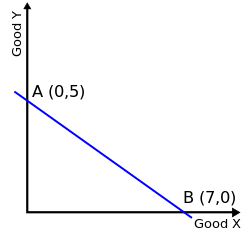
In economics, a budget constraint represents all the combinations of goods and services that a consumer may purchase given current prices within their given income. Consumer theory uses the concepts of a budget constraint and a preference map as tools to examine the parameters of consumer choices . Both concepts have a ready graphical representation in the two-good case. The consumer can only purchase as much as their income will allow, hence they are constrained by their budget. The equation of a budget constraint is ${\displaystyle P_{x}x+P_{y}y=m}$ where ${\displaystyle P_{x}}$ is the price of good X, and ${\displaystyle P_{y}}$ is the price of good Y, and m is income.

Soft budget constraint

The concept of soft budget constraint is commonly applied to economies in transition. This theory was originally proposed by János Kornai in 1979. It was used to explain the "economic behavior in socialist economies marked by shortage”. In the socialist transition economy there are soft budget constraint on firms because of subsidies, credit and price support. This theory implies that the survival of a firm depends on financial assistance, especially in a socialist country. The soft budget constraint syndrome usually occurs in the paternalistic role of the State in economic organizations, such as public and private companies and non-profit organizations. János Kornai also highlighted that there are five dimensions to evaluate the post-socialist transition, including fiscal subsidy, soft taxation, soft bank credit (non-performing loans), soft trade credit (the accumulate rears between firms) and wage arrears.

According to the point of view by Cllower , budget constraints are a rational planning assumption with two main attributes. The first is that budget constraints refer to the decision makers' behavioural characteristics --- selling output or acquiring asset income to compensate for spending. This means that adjustment limitation on financial resources are obvious. The second is to impose constraints on prior variables, such as constraints on current actual demand based on expectations of future financial conditions.

The reason for the soft budget constraints is that the excess of expenditure over income will be paid by additional organizations (the State). In addition, the decision maker expects such external financial assistance to be highly probable based on his actions. The further explanation is the more excess spending is covered by external aid, the budget constraints will be more softer.

Bank

Bank supervision refers to the supervision on the capital adequacy ratio of banks. When the bank's capital is difficult to finance due to the default of a large number of loans, it can prevent the bank from going bankrupt with the aid of the government, then it will occurs the soft budget constraint of the bank.

Dewatripont and Maskin(1995) point out the presence of sunk costs in existing loans may lead to soft budget constraints when banks need additional financial assistance. The internalization of external options can expand the model by allowing banks to allocate funds between new loans and refinancing old loans. Through investment screening and monitoring technology, banks can improve the relative profitability of new loans, thus breaking the equilibrium of soft budget constraints.

Uses

Individual choice

Consumer behaviour is a maximization problem. It means making the most of our limited resources to maximize our utility. As consumers are insatiable, and utility functions grow with quantity, the only thing that limits our consumption is our own budget.

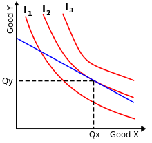
In general, the budget set (all bundle choices that are on or below the budget line) represents all possible bundles of goods an individual can afford given their income and the prices of goods. A common assumption underlying consumer theory is the concept of well-behaved preferences, and as such, the direction of an individual's preferences will point 45 degrees from the origin. When behaving rationally, an individual consumer should choose to consume goods at the point where the most preferred available indifference curve on their preference map is tangent to their budget constraint. The tangent point (the xy coordinate) represents the amount of goods x and y the consumer should purchase to fully utilize their budget to obtain maximum utility. It is important to note that the optimal consumption bundle will not always be an interior solution. If the solution to the optimality condition leads to a bundle that is not feasible, the consumer's optimal bundle will be a corner solution which suggests the goods or inputs are perfect substitutes. A line connecting all points of tangency between the indifference curve and the budget constraint is called the expansion path.

All two dimensional budget constraints are generalized into the equation:

${\displaystyle P_{x}x+P_{y}y=m}$

Where:

• ${\displaystyle m=}$ money income allocated to consumption (after saving and borrowing)
• ${\displaystyle P_{x}=}$ the price of a specific good
• ${\displaystyle P_{y}=}$ the price of all other goods
• ${\displaystyle x=}$ amount purchased of a specific good
• ${\displaystyle y=}$ amount purchased of all other goods

The equation can be rearranged to represent the shape of the curve on a graph:

${\displaystyle y=(m/P_{y})-(P_{x}/P_{y})x}$, where ${\displaystyle (m/P_{y})}$ is the y-intercept and ${\displaystyle (-P_{x}/P_{y})}$ is the slope, representing a downward sloping budget line.

The factors that can shift the budget line are a change in income (m), a change in the price of a specific good (${\displaystyle P_{x}}$), or a change in the price of all other goods (${\displaystyle P_{y}}$).

International economics

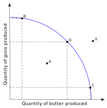
A production-possibility frontier is a constraint in some ways analogous to a budget constraint, showing limitations on a country's production of multiple goods based on the limitation of available factors of production. Under autarky this is also the limitation of consumption by individuals in the country. However, the benefits of international trade are generally demonstrated through allowance of a shift in the consumption-possibility frontiers of each trade partner which allows access to a more appealing indifference curve. In the "toolbox" Hecksher-Ohlin and Krugman models of international trade, the budget constraint of the economy (its CPF) is determined by the terms-of-trade (TOT) as a downward-sloped line with slope equal to those TOTs of the economy. (The TOTs are given by the price ratio Px/Py, where x is the exportable commodity and y is the importable).

Many goods

While low-level demonstrations of budget constraints are often limited to less than two good situations which provide easy graphical representation, it is possible to demonstrate the relationship between multiple goods through a budget constraint.

There are 2 requirements for this case. The first one is that the constraint is not affected if the prices are multiplied by any positive scalar. The second one is that all commodities are desirable and the constraint will always be binding.

In such a case, assuming there are ${\displaystyle n\,}$ goods, called ${\displaystyle x_{i}\,}$ for ${\displaystyle i=1,\dots ,n\,}$, that the price of good ${\displaystyle x_{i}\,}$ is denoted by ${\displaystyle p_{i}\,}$, and if ${\displaystyle \,W\,}$ is the total amount that may be spent, then the budget constraint is:

${\displaystyle \sum _{i=1}^{n}p_{i}x_{i}\leq W.}$

Further, if the consumer spends his income entirely, the budget constraint binds:

${\displaystyle \sum _{i=1}^{n}p_{i}x_{i}=W.}$

In this case, the consumer cannot obtain an additional unit of good ${\displaystyle x_{i}\,}$ without giving up some other good. For example, he could purchase an additional unit of good ${\displaystyle x_{i}\,}$ by giving up ${\displaystyle p_{i}/p_{j}\,}$ units of good ${\displaystyle x_{j}.\,}$

Borrowing and lending

Budget constraints can be expanded outward or contracted inward through borrowing and lending. By borrowing money in a period, usually at an interest rate r, a consumer can choose to forgo consumption in future periods for extra consumption in the borrowing period. Choosing to borrow would expand the budget constraint in this period and contract budget constraints in future periods. Alternatively, consumers can choose to lend their money in the current period, usually at a lending rate l. Lending contracts the budget constraint in the current period but expands budget constraints in future periods. According to behavioral economics, choices on borrowing and lending may also be affected by Present bias. In economics, there are two groups of present biased individuals, sophisticated individuals who are aware of their present bias, and naive individuals who are not aware of their present bias.

See also

• Choice modelling
• Contingent valuation
• Guns versus butter model
• Heckscher–Ohlin theorem on country level budget constraints called resource endowments
• Intertemporal budget constraint
• Isoquant
• Opportunity cost
• Scarcity
• Trade-off
• Paternalism

Notes

1. ^ Allingham, Michael (1987). Wealth Constraint, The New Palgrave: A Dictionary of Economics, doi:10.1057/978-1-349-95121-5_1886-1
2. Kornai, János; Maskin, Eric; Roland, Gérard (2003). "Understanding the Soft Budget Constraint". Journal of Economic Literature. 41 (4): 1095–1136. doi:10.1257/jel.41.4.1095. JSTOR 3217457.
3. Maskin, Eric; Xu, Chenggang (March 2001). "Soft budget constraint theories: From centralization to the market". The Economics of Transition. 9 (1): 1–27. doi:10.1111/1468-0351.00065. hdl:10722/138701. S2CID 154707861.
4. Vahabi, Mehrdad (2001). "The Soft Budget Constraint : A Theoretical Clarification" (PDF). Recherches Économiques de Louvain / Louvain Economic Review. 67 (2): 157–195. doi:10.1017/S0770451800055883. JSTOR 40724317. S2CID 152556966.
5. Kornai, János (February 1986). "The Soft Budget Constraint". Kyklos. 39 (1): 3–30. doi:10.1111/j.1467-6435.1986.tb01252.x.
6. Du, Julan; Li, David D. (March 2007). "The soft budget constraint of banks". Journal of Comparative Economics. 35 (1): 108–135. doi:10.1016/j.jce.2006.11.001.
7. Berglöf, Erik; Roland, Gérard (April 1997). "Soft budget constraints and credit crunches in financial transition". European Economic Review. 41 (3–5): 807–817. doi:10.1016/S0014-2921(97)00055-X.
8. "Budget constraint". Policonomics.
9. Lipsey (1975). p 182.
10. Salvatore, Dominick (1989). Schaum's outline of theory and problems of managerial economics, McGraw-Hill, ISBN 978-0-07-054513-7
11. O'Donoghue, Ted, and Matthew Rabin. 2015. "Present Bias: Lessons Learned and to Be Learned." American Economic Review, 105 (5): 273-79.

References

• Lipsey, Richard G. (1975). An Introduction to Positive Economics (Fourth ed.). Weidenfeld & Nicolson. pp. 214–7. ISBN 0-297-76899-9.
• Kornai, János; Maskin, Eric; Roland, Gérard (2003). "Understanding the Soft Budget Constraint". Journal of Economic Literature. 41 (4): 1095–1136. doi:10.1257/jel.41.4.1095. JSTOR 3217457.
• Vahabi, Mehrdad (2001). "The Soft Budget Constraint : A Theoretical Clarification" (PDF). Recherches Économiques de Louvain / Louvain Economic Review. 67 (2): 157–195. doi:10.1017/S0770451800055883. JSTOR 40724317. S2CID 152556966.
• Kornai, János (February 1986). "The Soft Budget Constraint". Kyklos. 39 (1): 3–30. doi:10.1111/j.1467-6435.1986.tb01252.x.
• Maskin, Eric; Xu, Chenggang (March 2001). "Soft budget constraint theories: From centralization to the market". The Economics of Transition. 9 (1): 1–27. doi:10.1111/1468-0351.00065. hdl:10722/138701. S2CID 154707861.
• Du, Julan; Li, David D. (March 2007). "The soft budget constraint of banks". Journal of Comparative Economics. 35 (1): 108–135. doi:10.1016/j.jce.2006.11.001.
• Berglöf, Erik; Roland, Gérard (April 1997). "Soft budget constraints and credit crunches in financial transition". European Economic Review. 41 (3–5): 807–817. doi:10.1016/S0014-2921(97)00055-X.

• Consumer theory
• Budgets
• Economics curves