Misplaced Pages

Schulz–Zimm

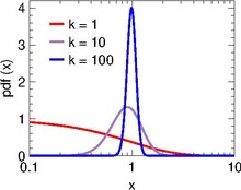
Probability density function
Parameters	${\displaystyle k}$ (shape parameter)
Support	${\displaystyle x\in \mathbb {R} _{>0}}$
PDF	${\displaystyle {\frac {k^{k}x^{k-1}e^{-kx}}{\Gamma (k)}}}$
Mean	${\displaystyle 1}$
Variance	${\displaystyle {\frac {1}{k}}}$

The Schulz–Zimm distribution is a special case of the gamma distribution. It is widely used to model the polydispersity of polymers. In this context it has been introduced in 1939 by Günter Victor Schulz and in 1948 by Bruno H. Zimm.

This distribution has only a shape parameter k, the scale being fixed at θ=1/k. Accordingly, the probability density function is $${\displaystyle f(x)={\frac {k^{k}x^{k-1}e^{-kx}}{\Gamma (k)}}.}$$

When applied to polymers, the variable x is the relative mass or chain length ${\displaystyle x=M/M_{n}}$. Accordingly, the mass distribution ${\displaystyle f(M)}$ is just a gamma distribution with scale parameter ${\displaystyle \theta =M_{n}/k}$. This explains why the Schulz–Zimm distribution is unheard of outside its conventional application domain.

The distribution has mean 1 and variance 1/k. The polymer dispersity is ${\displaystyle \langle x^{2}\rangle /\langle x\rangle =1+1/k}$.

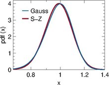
For large k the Schulz–Zimm distribution approaches a Gaussian distribution. In algorithms where one needs to draw samples ${\displaystyle x\geq 0}$, the Schulz–Zimm distribution is to be preferred over a Gaussian because the latter requires an arbitrary cut-off to prevent negative x.

References

1. G V Schulz (1939), Z. Phys. Chem. 43B, 25-46. - Eq (27a) with -ln(a), k+1 in place of our x,k.
2. B H Zimm (1948), J. Chem. Phys. 16, 1099. - Proposes a two-parameter variant of Eq (13) without derivation and without reference to Schulz or whomsoever. One of the two parameters can be eliminated by the requirement <n>=1.

• Continuous distributions