| This article needs additional citations for verification. Please help improve this article by adding citations to reliable sources. Unsourced material may be challenged and removed. Find sources: "Similarity" network science – news · newspapers · books · scholar · JSTOR (May 2014) (Learn how and when to remove this message) |
| Part of a series on | ||||
| Network science | ||||
|---|---|---|---|---|

| ||||
| Network types | ||||
| Graphs | ||||
|
||||
| Models | ||||
|
||||
| ||||
Similarity in network analysis occurs when two nodes (or other more elaborate structures) fall in the same equivalence class.
There are three fundamental approaches to constructing measures of network similarity: structural equivalence, automorphic equivalence, and regular equivalence. There is a hierarchy of the three equivalence concepts: any set of structural equivalences are also automorphic and regular equivalences. Any set of automorphic equivalences are also regular equivalences. Not all regular equivalences are necessarily automorphic or structural; and not all automorphic equivalences are necessarily structural.
Visualizing similarity and distance
Clustering tools
Agglomerative Hierarchical clustering of nodes on the basis of the similarity of their profiles of ties to other nodes provides a joining tree or Dendrogram that visualizes the degree of similarity among cases - and can be used to find approximate equivalence classes.
Multi-dimensional scaling tools
Main article: Multidimensional scalingUsually, our goal in equivalence analysis is to identify and visualize "classes" or clusters of cases. In using cluster analysis, we are implicitly assuming that the similarity or distance among cases reflects a single underlying dimension. It is possible, however, that there are multiple "aspects" or "dimensions" underlying the observed similarities of cases. Factor or components analysis could be applied to correlations or covariances among cases. Alternatively, multi-dimensional scaling could be used (non-metric for data that are inherently nominal or ordinal; metric for valued).
MDS represents the patterns of similarity or dissimilarity in the tie profiles among the actors (when applied to adjacency or distances) as a "map" in multi-dimensional space. This map lets us see how "close" actors are, whether they "cluster" in multi-dimensional space and how much variation there is along each dimension.
Structural equivalence
Two vertices of a network are structurally equivalent if they share many of the same neighbors.

There is no actor who has exactly the same set of ties as actor A, so actor A is in a class by itself. The same is true for actors B, C, D and G. Each of these nodes has a unique set of edges to other nodes. E and F, however, fall in the same structural equivalence class. Each has only one edge; and that tie is to B. Since E and F have exactly the same pattern of edges with all the vertices, they are structurally equivalent. The same is true in the case of H and I.
Structural equivalence is the strongest form of similarity. In many real networks, exact equivalence may be rare, and it could be useful to ease the criteria and measure approximate equivalence.
A closely related concept is institutional equivalence: two actors (e.g., firms) are institutionally equivalent if they operate in the same set of institutional fields. While structurally equivalent actors have identical relational patterns or network positions, institutional equivalence captures the similarity of institutional influences that actors experience from being in the same fields, regardless of how similar their network positions are. For example, two banks in Chicago might have very different patterns of ties (e.g., one may be a central node, and the other may be in a peripheral position) such that they are not structural equivalents, but because they both operate in the field of finance and banking and in the same geographically defined field (Chicago), they will be subject to some of the same institutional influences.
Measures for structural equivalence
Cosine similarity
Main article: Cosine similarityA simple count of common neighbors for two vertices is not on its own a very good measure. One should know the degree of the vertices or how many common neighbors other pairs of vertices has. Cosine similarity takes into account these regards and also allow for varying degrees of vertices. Salton proposed that we regard the i-th and j-th rows/columns of the adjacency matrix as two vectors and use the cosine of the angle between them as a similarity measure. The cosine similarity of i and j is the number of common neighbors divided by the geometric mean of their degrees.
Its value lies in the range from 0 to 1. The value of 1 indicates that the two vertices have exactly the same neighbors while the value of zero means that they do not have any common neighbors. Cosine similarity is technically undefined if one or both of the nodes has zero degree, but according to the convention, we say that cosine similarity is 0 in these cases.
Pearson coefficient
Main article: Pearson product-moment correlation coefficientPearson product-moment correlation coefficient is an alternative method to normalize the count of common neighbors. This method compares the number of common neighbors with the expected value that count would take in a network where vertices are connected randomly. This quantity lies strictly in the range from -1 to 1.
Euclidean distance
Main article: Euclidean distanceEuclidean distance is equal to the number of neighbors that differ between two vertices. It is rather a dissimilarity measure, since it is larger for vertices which differ more. It could be normalized by dividing by its maximum value. The maximum means that there are no common neighbors, in which case the distance is equal to the sum of the degrees of the vertices.
Automorphic equivalence
Formally "Two vertices are automorphically equivalent if all the vertices can be re-labeled to form an isomorphic graph with the labels of u and v interchanged. Two automorphically equivalent vertices share exactly the same label-independent properties."
More intuitively, actors are automorphically equivalent if we can permute the graph in such a way that exchanging the two actors has no effect on the distances among all actors in the graph.

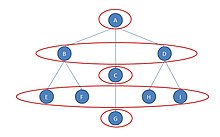
Suppose the graph describes the organizational structure of a company. Actor A is the central headquarter, actors B, C, and D are managers. Actors E, F and H, I are workers at smaller stores; G is the lone worker at another store.
Even though actor B and actor D are not structurally equivalent (they do have the same boss, but not the same workers), they do seem to be "equivalent" in a different sense. Both manager B and D have a boss (in this case, the same boss), and each has two workers. If we swapped them, and also swapped the four workers, all of the distances among all the actors in the network would be exactly identical.
There are actually five automorphic equivalence classes: {A}, {B, D}, {C}, {E, F, H, I}, and {G}. Note that the less strict definition of "equivalence" has reduced the number of classes.
Regular equivalence
Formally, "Two actors are regularly equivalent if they are equally related to equivalent others." In other words, regularly equivalent vertices are vertices that, while they do not necessarily share neighbors, have neighbors who are themselves similar.
Two mothers, for example, are equivalent, because each has a similar pattern of connections with a husband, children, etc. The two mothers do not have ties to the same husband or the same children, so they are not structurally equivalent. Because different mothers may have different numbers of husbands and children, they will not be automorphically equivalent. But they are similar because they have the same relationships with some member or members of another set of actors (who are themselves regarded as equivalent because of the similarity of their ties to a member of the set "mother").

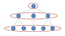
In the graph there are three regular equivalence classes. The first is actor A; the second is composed of the three actors B, C, and D; the third consists of the remaining five actors E, F, G, H, and I.
The easiest class to see is the five actors across the bottom of the diagram (E, F, G, H, and I). These actors are regularly equivalent to one another because:
- they have no tie with any actor in the first class (that is, with actor A) and
- each has a tie with an actor in the second class (either B or C or D).
Each of the five actors, then, has an identical pattern of ties with actors in the other classes.
Actors B, C, and D form a class similarly. B and D actually have ties with two members of the third class, whereas actor C has a tie to only one member of the third class, but this doesn't matter, as there is a tie to some member of the third class.
Actor A is in a class by itself, defined by:
- a tie to at least one member of class two and
- no tie to any member of class three.
See also
References
- ^ Newman, M.E.J. 2010. Networks: An Introduction. Oxford, UK: Oxford University Press.
- ^ Hanneman, Robert A. and Mark Riddle. 2005. Introduction to social network methods. Riverside, CA: University of California, Riverside ( published in digital form at http://faculty.ucr.edu/~hanneman/ )
- ^ Marquis, Christopher; Tilcsik, András (2016-10-01). "Institutional Equivalence: How Industry and Community Peers Influence Corporate Philanthropy". Organization Science. 27 (5): 1325–1341. doi:10.1287/orsc.2016.1083. hdl:1813/44734. ISSN 1047-7039.
- Salton G., Automatic Text Processing: The Transformation, Analysis and Retrieval of Information by Computer, Addison-Wesley, Reading, MA (1989)
- ^ Borgatti, Steven, Martin Everett, and Linton Freeman. 1992. UCINET IV Version 1.0 User's Guide. Columbia, SC: Analytic Technologies.