Misplaced Pages

Shear modulus

Article snapshot taken from Wikipedia with creative commons attribution-sharealike license. Give it a read and then ask your questions in the chat. We can research this topic together.
(Redirected from Modulus rigidity) Ratio of shear stress to shear strain
Shear modulus
Common symbolsG, S, μ
SI unitPa
Derivations from
other quantities
G = τ / γ = E /
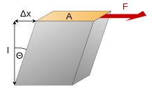
Shear strain

In materials science, shear modulus or modulus of rigidity, denoted by G, or sometimes S or μ, is a measure of the elastic shear stiffness of a material and is defined as the ratio of shear stress to the shear strain:

G   = d e f   τ x y γ x y = F / A Δ x / l = F l A Δ x {\displaystyle G\ {\stackrel {\mathrm {def} }{=}}\ {\frac {\tau _{xy}}{\gamma _{xy}}}={\frac {F/A}{\Delta x/l}}={\frac {Fl}{A\Delta x}}}

where

τ x y = F / A {\displaystyle \tau _{xy}=F/A\,} = shear stress
F {\displaystyle F} is the force which acts
A {\displaystyle A} is the area on which the force acts
γ x y {\displaystyle \gamma _{xy}} = shear strain. In engineering := Δ x / l = tan θ {\displaystyle :=\Delta x/l=\tan \theta } , elsewhere := θ {\displaystyle :=\theta }
Δ x {\displaystyle \Delta x} is the transverse displacement
l {\displaystyle l} is the initial length of the area.

The derived SI unit of shear modulus is the pascal (Pa), although it is usually expressed in gigapascals (GPa) or in thousand pounds per square inch (ksi). Its dimensional form is MLT, replacing force by mass times acceleration.

Explanation

Material Typical values for
shear modulus (GPa)
(at room temperature)
Diamond 478.0
Steel 79.3
Iron 52.5
Copper 44.7
Titanium 41.4
Glass 26.2
Aluminium 25.5
Polyethylene 0.117
Rubber 0.0006
Granite 24
Shale 1.6
Limestone 24
Chalk 3.2
Sandstone 0.4
Wood 4

The shear modulus is one of several quantities for measuring the stiffness of materials. All of them arise in the generalized Hooke's law:

  • Young's modulus E describes the material's strain response to uniaxial stress in the direction of this stress (like pulling on the ends of a wire or putting a weight on top of a column, with the wire getting longer and the column losing height),
  • the Poisson's ratio ν describes the response in the directions orthogonal to this uniaxial stress (the wire getting thinner and the column thicker),
  • the bulk modulus K describes the material's response to (uniform) hydrostatic pressure (like the pressure at the bottom of the ocean or a deep swimming pool),
  • the shear modulus G describes the material's response to shear stress (like cutting it with dull scissors).

These moduli are not independent, and for isotropic materials they are connected via the equations

E = 2 G ( 1 + ν ) = 3 K ( 1 2 ν ) {\displaystyle E=2G(1+\nu )=3K(1-2\nu )}

The shear modulus is concerned with the deformation of a solid when it experiences a force parallel to one of its surfaces while its opposite face experiences an opposing force (such as friction). In the case of an object shaped like a rectangular prism, it will deform into a parallelepiped. Anisotropic materials such as wood, paper and also essentially all single crystals exhibit differing material response to stress or strain when tested in different directions. In this case, one may need to use the full tensor-expression of the elastic constants, rather than a single scalar value.

One possible definition of a fluid would be a material with zero shear modulus.

Shear waves

Influences of selected glass component additions on the shear modulus of a specific base glass.

In homogeneous and isotropic solids, there are two kinds of waves, pressure waves and shear waves. The velocity of a shear wave, ( v s ) {\displaystyle (v_{s})} is controlled by the shear modulus,

v s = G ρ {\displaystyle v_{s}={\sqrt {\frac {G}{\rho }}}}

where

G is the shear modulus
ρ {\displaystyle \rho } is the solid's density.

Shear modulus of metals
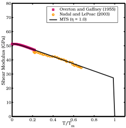
Shear modulus of copper as a function of temperature. The experimental data are shown with colored symbols.

The shear modulus of metals is usually observed to decrease with increasing temperature. At high pressures, the shear modulus also appears to increase with the applied pressure. Correlations between the melting temperature, vacancy formation energy, and the shear modulus have been observed in many metals.

Several models exist that attempt to predict the shear modulus of metals (and possibly that of alloys). Shear modulus models that have been used in plastic flow computations include:

  1. the Varshni-Chen-Gray model developed by and used in conjunction with the Mechanical Threshold Stress (MTS) plastic flow stress model.
  2. the Steinberg-Cochran-Guinan (SCG) shear modulus model developed by and used in conjunction with the Steinberg-Cochran-Guinan-Lund (SCGL) flow stress model.
  3. the Nadal and LePoac (NP) shear modulus model that uses Lindemann theory to determine the temperature dependence and the SCG model for pressure dependence of the shear modulus.

Varshni-Chen-Gray model

The Varshni-Chen-Gray model (sometimes referred to as the Varshni equation) has the form:

μ ( T ) = μ 0 D exp ( T 0 / T ) 1 {\displaystyle \mu (T)=\mu _{0}-{\frac {D}{\exp(T_{0}/T)-1}}}

where μ 0 {\displaystyle \mu _{0}} is the shear modulus at T = 0 K {\displaystyle T=0K} , and D {\displaystyle D} and T 0 {\displaystyle T_{0}} are material constants.

SCG model

The Steinberg-Cochran-Guinan (SCG) shear modulus model is pressure dependent and has the form

μ ( p , T ) = μ 0 + μ p p η 1 3 + μ T ( T 300 ) ; η := ρ ρ 0 {\displaystyle \mu (p,T)=\mu _{0}+{\frac {\partial \mu }{\partial p}}{\frac {p}{\eta ^{\frac {1}{3}}}}+{\frac {\partial \mu }{\partial T}}(T-300);\quad \eta :={\frac {\rho }{\rho _{0}}}}

where, μ0 is the shear modulus at the reference state (T = 300 K, p = 0, η = 1), p is the pressure, and T is the temperature.

NP model

The Nadal-Le Poac (NP) shear modulus model is a modified version of the SCG model. The empirical temperature dependence of the shear modulus in the SCG model is replaced with an equation based on Lindemann melting theory. The NP shear modulus model has the form:

μ ( p , T ) = 1 J ( T ^ ) [ ( μ 0 + μ p p η 1 3 ) ( 1 T ^ ) + ρ C m   T ] ; C := ( 6 π 2 ) 2 3 3 f 2 {\displaystyle \mu (p,T)={\frac {1}{{\mathcal {J}}\left({\hat {T}}\right)}}\left;\quad C:={\frac {\left(6\pi ^{2}\right)^{\frac {2}{3}}}{3}}f^{2}}

where

J ( T ^ ) := 1 + exp [ 1 + 1 / ζ 1 + ζ / ( 1 T ^ ) ] for T ^ := T T m [ 0 , 6 + ζ ] , {\displaystyle {\mathcal {J}}({\hat {T}}):=1+\exp \left\quad {\text{for}}\quad {\hat {T}}:={\frac {T}{T_{m}}}\in ,}

and μ0 is the shear modulus at absolute zero and ambient pressure, ζ is an area, m is the atomic mass, and f is the Lindemann constant.

Shear relaxation modulus

The shear relaxation modulus G ( t ) {\displaystyle G(t)} is the time-dependent generalization of the shear modulus G {\displaystyle G} :

G = lim t G ( t ) {\displaystyle G=\lim _{t\to \infty }G(t)} .

See also

References

  1. IUPAC, Compendium of Chemical Terminology, 2nd ed. (the "Gold Book") (1997). Online corrected version: (2006–) "shear modulus, G". doi:10.1351/goldbook.S05635
  2. McSkimin, H.J.; Andreatch, P. (1972). "Elastic Moduli of Diamond as a Function of Pressure and Temperature". J. Appl. Phys. 43 (7): 2944–2948. Bibcode:1972JAP....43.2944M. doi:10.1063/1.1661636.
  3. ^ Crandall, Dahl, Lardner (1959). An Introduction to the Mechanics of Solids. Boston: McGraw-Hill. ISBN 0-07-013441-3.{{cite book}}: CS1 maint: multiple names: authors list (link)
  4. Rayne, J.A. (1961). "Elastic constants of Iron from 4.2 to 300 ° K". Physical Review. 122 (6): 1714–1716. Bibcode:1961PhRv..122.1714R. doi:10.1103/PhysRev.122.1714.
  5. Material properties
  6. Spanos, Pete (2003). "Cure system effect on low temperature dynamic shear modulus of natural rubber". Rubber World.
  7. ^ Hoek, Evert, and Jonathan D. Bray. Rock slope engineering. CRC Press, 1981.
  8. ^ Pariseau, William G. Design analysis in rock mechanics. CRC Press, 2017.
  9. Shear modulus calculation of glasses
  10. Overton, W.; Gaffney, John (1955). "Temperature Variation of the Elastic Constants of Cubic Elements. I. Copper". Physical Review. 98 (4): 969. Bibcode:1955PhRv...98..969O. doi:10.1103/PhysRev.98.969.
  11. ^ Nadal, Marie-Hélène; Le Poac, Philippe (2003). "Continuous model for the shear modulus as a function of pressure and temperature up to the melting point: Analysis and ultrasonic validation". Journal of Applied Physics. 93 (5): 2472. Bibcode:2003JAP....93.2472N. doi:10.1063/1.1539913.
  12. March, N. H., (1996), Electron Correlation in Molecules and Condensed Phases, Springer, ISBN 0-306-44844-0 p. 363
  13. Varshni, Y. (1970). "Temperature Dependence of the Elastic Constants". Physical Review B. 2 (10): 3952–3958. Bibcode:1970PhRvB...2.3952V. doi:10.1103/PhysRevB.2.3952.
  14. Chen, Shuh Rong; Gray, George T. (1996). "Constitutive behavior of tantalum and tantalum-tungsten alloys". Metallurgical and Materials Transactions A. 27 (10): 2994. Bibcode:1996MMTA...27.2994C. doi:10.1007/BF02663849. S2CID 136695336.
  15. Goto, D. M.; Garrett, R. K.; Bingert, J. F.; Chen, S. R.; Gray, G. T. (2000). "The mechanical threshold stress constitutive-strength model description of HY-100 steel" (PDF). Metallurgical and Materials Transactions A. 31 (8): 1985–1996. Bibcode:2000MMTA...31.1985G. doi:10.1007/s11661-000-0226-8. S2CID 136118687. Archived from the original on September 25, 2017.
  16. Guinan, M; Steinberg, D (1974). "Pressure and temperature derivatives of the isotropic polycrystalline shear modulus for 65 elements". Journal of Physics and Chemistry of Solids. 35 (11): 1501. Bibcode:1974JPCS...35.1501G. doi:10.1016/S0022-3697(74)80278-7.
  17. Rubinstein, Michael, 1956 December 20- (2003). Polymer physics. Colby, Ralph H. Oxford: Oxford University Press. p. 284. ISBN 019852059X. OCLC 50339757.{{cite book}}: CS1 maint: multiple names: authors list (link) CS1 maint: numeric names: authors list (link)
Elastic moduli for homogeneous isotropic materials
Conversion formulae
Homogeneous isotropic linear elastic materials have their elastic properties uniquely determined by any two moduli among these; thus, given any two, any other of the elastic moduli can be calculated according to these formulas, provided both for 3D materials (first part of the table) and for 2D materials (second part).
3D formulae K = {\displaystyle K=\,} E = {\displaystyle E=\,} λ = {\displaystyle \lambda =\,} G = {\displaystyle G=\,} ν = {\displaystyle \nu =\,} M = {\displaystyle M=\,} Notes
( K , E ) {\displaystyle (K,\,E)} 3 K ( 3 K E ) 9 K E {\displaystyle {\tfrac {3K(3K-E)}{9K-E}}} 3 K E 9 K E {\displaystyle {\tfrac {3KE}{9K-E}}} 3 K E 6 K {\displaystyle {\tfrac {3K-E}{6K}}} 3 K ( 3 K + E ) 9 K E {\displaystyle {\tfrac {3K(3K+E)}{9K-E}}}
( K , λ ) {\displaystyle (K,\,\lambda )} 9 K ( K λ ) 3 K λ {\displaystyle {\tfrac {9K(K-\lambda )}{3K-\lambda }}} 3 ( K λ ) 2 {\displaystyle {\tfrac {3(K-\lambda )}{2}}} λ 3 K λ {\displaystyle {\tfrac {\lambda }{3K-\lambda }}} 3 K 2 λ {\displaystyle 3K-2\lambda \,}
( K , G ) {\displaystyle (K,\,G)} 9 K G 3 K + G {\displaystyle {\tfrac {9KG}{3K+G}}} K 2 G 3 {\displaystyle K-{\tfrac {2G}{3}}} 3 K 2 G 2 ( 3 K + G ) {\displaystyle {\tfrac {3K-2G}{2(3K+G)}}} K + 4 G 3 {\displaystyle K+{\tfrac {4G}{3}}}
( K , ν ) {\displaystyle (K,\,\nu )} 3 K ( 1 2 ν ) {\displaystyle 3K(1-2\nu )\,} 3 K ν 1 + ν {\displaystyle {\tfrac {3K\nu }{1+\nu }}} 3 K ( 1 2 ν ) 2 ( 1 + ν ) {\displaystyle {\tfrac {3K(1-2\nu )}{2(1+\nu )}}} 3 K ( 1 ν ) 1 + ν {\displaystyle {\tfrac {3K(1-\nu )}{1+\nu }}}
( K , M ) {\displaystyle (K,\,M)} 9 K ( M K ) 3 K + M {\displaystyle {\tfrac {9K(M-K)}{3K+M}}} 3 K M 2 {\displaystyle {\tfrac {3K-M}{2}}} 3 ( M K ) 4 {\displaystyle {\tfrac {3(M-K)}{4}}} 3 K M 3 K + M {\displaystyle {\tfrac {3K-M}{3K+M}}}
( E , λ ) {\displaystyle (E,\,\lambda )} E + 3 λ + R 6 {\displaystyle {\tfrac {E+3\lambda +R}{6}}} E 3 λ + R 4 {\displaystyle {\tfrac {E-3\lambda +R}{4}}} 2 λ E + λ + R {\displaystyle {\tfrac {2\lambda }{E+\lambda +R}}} E λ + R 2 {\displaystyle {\tfrac {E-\lambda +R}{2}}} R = E 2 + 9 λ 2 + 2 E λ {\displaystyle R={\sqrt {E^{2}+9\lambda ^{2}+2E\lambda }}}
( E , G ) {\displaystyle (E,\,G)} E G 3 ( 3 G E ) {\displaystyle {\tfrac {EG}{3(3G-E)}}} G ( E 2 G ) 3 G E {\displaystyle {\tfrac {G(E-2G)}{3G-E}}} E 2 G 1 {\displaystyle {\tfrac {E}{2G}}-1} G ( 4 G E ) 3 G E {\displaystyle {\tfrac {G(4G-E)}{3G-E}}}
( E , ν ) {\displaystyle (E,\,\nu )} E 3 ( 1 2 ν ) {\displaystyle {\tfrac {E}{3(1-2\nu )}}} E ν ( 1 + ν ) ( 1 2 ν ) {\displaystyle {\tfrac {E\nu }{(1+\nu )(1-2\nu )}}} E 2 ( 1 + ν ) {\displaystyle {\tfrac {E}{2(1+\nu )}}} E ( 1 ν ) ( 1 + ν ) ( 1 2 ν ) {\displaystyle {\tfrac {E(1-\nu )}{(1+\nu )(1-2\nu )}}}
( E , M ) {\displaystyle (E,\,M)} 3 M E + S 6 {\displaystyle {\tfrac {3M-E+S}{6}}} M E + S 4 {\displaystyle {\tfrac {M-E+S}{4}}} 3 M + E S 8 {\displaystyle {\tfrac {3M+E-S}{8}}} E M + S 4 M {\displaystyle {\tfrac {E-M+S}{4M}}} S = ± E 2 + 9 M 2 10 E M {\displaystyle S=\pm {\sqrt {E^{2}+9M^{2}-10EM}}}

There are two valid solutions.
The plus sign leads to ν 0 {\displaystyle \nu \geq 0} .

The minus sign leads to ν 0 {\displaystyle \nu \leq 0} .

( λ , G ) {\displaystyle (\lambda ,\,G)} λ + 2 G 3 {\displaystyle \lambda +{\tfrac {2G}{3}}} G ( 3 λ + 2 G ) λ + G {\displaystyle {\tfrac {G(3\lambda +2G)}{\lambda +G}}} λ 2 ( λ + G ) {\displaystyle {\tfrac {\lambda }{2(\lambda +G)}}} λ + 2 G {\displaystyle \lambda +2G\,}
( λ , ν ) {\displaystyle (\lambda ,\,\nu )} λ ( 1 + ν ) 3 ν {\displaystyle {\tfrac {\lambda (1+\nu )}{3\nu }}} λ ( 1 + ν ) ( 1 2 ν ) ν {\displaystyle {\tfrac {\lambda (1+\nu )(1-2\nu )}{\nu }}} λ ( 1 2 ν ) 2 ν {\displaystyle {\tfrac {\lambda (1-2\nu )}{2\nu }}} λ ( 1 ν ) ν {\displaystyle {\tfrac {\lambda (1-\nu )}{\nu }}} Cannot be used when ν = 0 λ = 0 {\displaystyle \nu =0\Leftrightarrow \lambda =0}
( λ , M ) {\displaystyle (\lambda ,\,M)} M + 2 λ 3 {\displaystyle {\tfrac {M+2\lambda }{3}}} ( M λ ) ( M + 2 λ ) M + λ {\displaystyle {\tfrac {(M-\lambda )(M+2\lambda )}{M+\lambda }}} M λ 2 {\displaystyle {\tfrac {M-\lambda }{2}}} λ M + λ {\displaystyle {\tfrac {\lambda }{M+\lambda }}}
( G , ν ) {\displaystyle (G,\,\nu )} 2 G ( 1 + ν ) 3 ( 1 2 ν ) {\displaystyle {\tfrac {2G(1+\nu )}{3(1-2\nu )}}} 2 G ( 1 + ν ) {\displaystyle 2G(1+\nu )\,} 2 G ν 1 2 ν {\displaystyle {\tfrac {2G\nu }{1-2\nu }}} 2 G ( 1 ν ) 1 2 ν {\displaystyle {\tfrac {2G(1-\nu )}{1-2\nu }}}
( G , M ) {\displaystyle (G,\,M)} M 4 G 3 {\displaystyle M-{\tfrac {4G}{3}}} G ( 3 M 4 G ) M G {\displaystyle {\tfrac {G(3M-4G)}{M-G}}} M 2 G {\displaystyle M-2G\,} M 2 G 2 M 2 G {\displaystyle {\tfrac {M-2G}{2M-2G}}}
( ν , M ) {\displaystyle (\nu ,\,M)} M ( 1 + ν ) 3 ( 1 ν ) {\displaystyle {\tfrac {M(1+\nu )}{3(1-\nu )}}} M ( 1 + ν ) ( 1 2 ν ) 1 ν {\displaystyle {\tfrac {M(1+\nu )(1-2\nu )}{1-\nu }}} M ν 1 ν {\displaystyle {\tfrac {M\nu }{1-\nu }}} M ( 1 2 ν ) 2 ( 1 ν ) {\displaystyle {\tfrac {M(1-2\nu )}{2(1-\nu )}}}
2D formulae K 2 D = {\displaystyle K_{\mathrm {2D} }=\,} E 2 D = {\displaystyle E_{\mathrm {2D} }=\,} λ 2 D = {\displaystyle \lambda _{\mathrm {2D} }=\,} G 2 D = {\displaystyle G_{\mathrm {2D} }=\,} ν 2 D = {\displaystyle \nu _{\mathrm {2D} }=\,} M 2 D = {\displaystyle M_{\mathrm {2D} }=\,} Notes
( K 2 D , E 2 D ) {\displaystyle (K_{\mathrm {2D} },\,E_{\mathrm {2D} })} 2 K 2 D ( 2 K 2 D E 2 D ) 4 K 2 D E 2 D {\displaystyle {\tfrac {2K_{\mathrm {2D} }(2K_{\mathrm {2D} }-E_{\mathrm {2D} })}{4K_{\mathrm {2D} }-E_{\mathrm {2D} }}}} K 2 D E 2 D 4 K 2 D E 2 D {\displaystyle {\tfrac {K_{\mathrm {2D} }E_{\mathrm {2D} }}{4K_{\mathrm {2D} }-E_{\mathrm {2D} }}}} 2 K 2 D E 2 D 2 K 2 D {\displaystyle {\tfrac {2K_{\mathrm {2D} }-E_{\mathrm {2D} }}{2K_{\mathrm {2D} }}}} 4 K 2 D 2 4 K 2 D E 2 D {\displaystyle {\tfrac {4K_{\mathrm {2D} }^{2}}{4K_{\mathrm {2D} }-E_{\mathrm {2D} }}}}
( K 2 D , λ 2 D ) {\displaystyle (K_{\mathrm {2D} },\,\lambda _{\mathrm {2D} })} 4 K 2 D ( K 2 D λ 2 D ) 2 K 2 D λ 2 D {\displaystyle {\tfrac {4K_{\mathrm {2D} }(K_{\mathrm {2D} }-\lambda _{\mathrm {2D} })}{2K_{\mathrm {2D} }-\lambda _{\mathrm {2D} }}}} K 2 D λ 2 D {\displaystyle K_{\mathrm {2D} }-\lambda _{\mathrm {2D} }} λ 2 D 2 K 2 D λ 2 D {\displaystyle {\tfrac {\lambda _{\mathrm {2D} }}{2K_{\mathrm {2D} }-\lambda _{\mathrm {2D} }}}} 2 K 2 D λ 2 D {\displaystyle 2K_{\mathrm {2D} }-\lambda _{\mathrm {2D} }}
( K 2 D , G 2 D ) {\displaystyle (K_{\mathrm {2D} },\,G_{\mathrm {2D} })} 4 K 2 D G 2 D K 2 D + G 2 D {\displaystyle {\tfrac {4K_{\mathrm {2D} }G_{\mathrm {2D} }}{K_{\mathrm {2D} }+G_{\mathrm {2D} }}}} K 2 D G 2 D {\displaystyle K_{\mathrm {2D} }-G_{\mathrm {2D} }} K 2 D G 2 D K 2 D + G 2 D {\displaystyle {\tfrac {K_{\mathrm {2D} }-G_{\mathrm {2D} }}{K_{\mathrm {2D} }+G_{\mathrm {2D} }}}} K 2 D + G 2 D {\displaystyle K_{\mathrm {2D} }+G_{\mathrm {2D} }}
( K 2 D , ν 2 D ) {\displaystyle (K_{\mathrm {2D} },\,\nu _{\mathrm {2D} })} 2 K 2 D ( 1 ν 2 D ) {\displaystyle 2K_{\mathrm {2D} }(1-\nu _{\mathrm {2D} })\,} 2 K 2 D ν 2 D 1 + ν 2 D {\displaystyle {\tfrac {2K_{\mathrm {2D} }\nu _{\mathrm {2D} }}{1+\nu _{\mathrm {2D} }}}} K 2 D ( 1 ν 2 D ) 1 + ν 2 D {\displaystyle {\tfrac {K_{\mathrm {2D} }(1-\nu _{\mathrm {2D} })}{1+\nu _{\mathrm {2D} }}}} 2 K 2 D 1 + ν 2 D {\displaystyle {\tfrac {2K_{\mathrm {2D} }}{1+\nu _{\mathrm {2D} }}}}
( E 2 D , G 2 D ) {\displaystyle (E_{\mathrm {2D} },\,G_{\mathrm {2D} })} E 2 D G 2 D 4 G 2 D E 2 D {\displaystyle {\tfrac {E_{\mathrm {2D} }G_{\mathrm {2D} }}{4G_{\mathrm {2D} }-E_{\mathrm {2D} }}}} 2 G 2 D ( E 2 D 2 G 2 D ) 4 G 2 D E 2 D {\displaystyle {\tfrac {2G_{\mathrm {2D} }(E_{\mathrm {2D} }-2G_{\mathrm {2D} })}{4G_{\mathrm {2D} }-E_{\mathrm {2D} }}}} E 2 D 2 G 2 D 1 {\displaystyle {\tfrac {E_{\mathrm {2D} }}{2G_{\mathrm {2D} }}}-1} 4 G 2 D 2 4 G 2 D E 2 D {\displaystyle {\tfrac {4G_{\mathrm {2D} }^{2}}{4G_{\mathrm {2D} }-E_{\mathrm {2D} }}}}
( E 2 D , ν 2 D ) {\displaystyle (E_{\mathrm {2D} },\,\nu _{\mathrm {2D} })} E 2 D 2 ( 1 ν 2 D ) {\displaystyle {\tfrac {E_{\mathrm {2D} }}{2(1-\nu _{\mathrm {2D} })}}} E 2 D ν 2 D ( 1 + ν 2 D ) ( 1 ν 2 D ) {\displaystyle {\tfrac {E_{\mathrm {2D} }\nu _{\mathrm {2D} }}{(1+\nu _{\mathrm {2D} })(1-\nu _{\mathrm {2D} })}}} E 2 D 2 ( 1 + ν 2 D ) {\displaystyle {\tfrac {E_{\mathrm {2D} }}{2(1+\nu _{\mathrm {2D} })}}} E 2 D ( 1 + ν 2 D ) ( 1 ν 2 D ) {\displaystyle {\tfrac {E_{\mathrm {2D} }}{(1+\nu _{\mathrm {2D} })(1-\nu _{\mathrm {2D} })}}}
( λ 2 D , G 2 D ) {\displaystyle (\lambda _{\mathrm {2D} },\,G_{\mathrm {2D} })} λ 2 D + G 2 D {\displaystyle \lambda _{\mathrm {2D} }+G_{\mathrm {2D} }} 4 G 2 D ( λ 2 D + G 2 D ) λ 2 D + 2 G 2 D {\displaystyle {\tfrac {4G_{\mathrm {2D} }(\lambda _{\mathrm {2D} }+G_{\mathrm {2D} })}{\lambda _{\mathrm {2D} }+2G_{\mathrm {2D} }}}} λ 2 D λ 2 D + 2 G 2 D {\displaystyle {\tfrac {\lambda _{\mathrm {2D} }}{\lambda _{\mathrm {2D} }+2G_{\mathrm {2D} }}}} λ 2 D + 2 G 2 D {\displaystyle \lambda _{\mathrm {2D} }+2G_{\mathrm {2D} }\,}
( λ 2 D , ν 2 D ) {\displaystyle (\lambda _{\mathrm {2D} },\,\nu _{\mathrm {2D} })} λ 2 D ( 1 + ν 2 D ) 2 ν 2 D {\displaystyle {\tfrac {\lambda _{\mathrm {2D} }(1+\nu _{\mathrm {2D} })}{2\nu _{\mathrm {2D} }}}} λ 2 D ( 1 + ν 2 D ) ( 1 ν 2 D ) ν 2 D {\displaystyle {\tfrac {\lambda _{\mathrm {2D} }(1+\nu _{\mathrm {2D} })(1-\nu _{\mathrm {2D} })}{\nu _{\mathrm {2D} }}}} λ 2 D ( 1 ν 2 D ) 2 ν 2 D {\displaystyle {\tfrac {\lambda _{\mathrm {2D} }(1-\nu _{\mathrm {2D} })}{2\nu _{\mathrm {2D} }}}} λ 2 D ν 2 D {\displaystyle {\tfrac {\lambda _{\mathrm {2D} }}{\nu _{\mathrm {2D} }}}} Cannot be used when ν 2 D = 0 λ 2 D = 0 {\displaystyle \nu _{\mathrm {2D} }=0\Leftrightarrow \lambda _{\mathrm {2D} }=0}
( G 2 D , ν 2 D ) {\displaystyle (G_{\mathrm {2D} },\,\nu _{\mathrm {2D} })} G 2 D ( 1 + ν 2 D ) 1 ν 2 D {\displaystyle {\tfrac {G_{\mathrm {2D} }(1+\nu _{\mathrm {2D} })}{1-\nu _{\mathrm {2D} }}}} 2 G 2 D ( 1 + ν 2 D ) {\displaystyle 2G_{\mathrm {2D} }(1+\nu _{\mathrm {2D} })\,} 2 G 2 D ν 2 D 1 ν 2 D {\displaystyle {\tfrac {2G_{\mathrm {2D} }\nu _{\mathrm {2D} }}{1-\nu _{\mathrm {2D} }}}} 2 G 2 D 1 ν 2 D {\displaystyle {\tfrac {2G_{\mathrm {2D} }}{1-\nu _{\mathrm {2D} }}}}
( G 2 D , M 2 D ) {\displaystyle (G_{\mathrm {2D} },\,M_{\mathrm {2D} })} M 2 D G 2 D {\displaystyle M_{\mathrm {2D} }-G_{\mathrm {2D} }} 4 G 2 D ( M 2 D G 2 D ) M 2 D {\displaystyle {\tfrac {4G_{\mathrm {2D} }(M_{\mathrm {2D} }-G_{\mathrm {2D} })}{M_{\mathrm {2D} }}}} M 2 D 2 G 2 D {\displaystyle M_{\mathrm {2D} }-2G_{\mathrm {2D} }\,} M 2 D 2 G 2 D M 2 D {\displaystyle {\tfrac {M_{\mathrm {2D} }-2G_{\mathrm {2D} }}{M_{\mathrm {2D} }}}}


Categories: